This appendix briefly reviews the most common methods for solving ordinary differential equations (ODEs). Many ODEs or systems of ODEs introduced in these notes are nonlinear and cannot therefore be easily solved with such methods. However, linear stability analysis of fixed points relies on solving linear systems with constant coefficients, which are discussed here. Moreover, it is essential for a modeler to be able to recognize ODEs that can be solved exactly, and to solve them if necessary. The information below is meant to be used as a quick reference; theorems are given without proof and the reader should consult classical texts on differential equations for details.

Definitions and basic existence theorems

Definitions

• An ordinary differential equation of order [latex]n[/latex] is an equation of the form

[latex]\displaystyle \frac{d^n y}{d x^n}=F\left( x,y,\frac{d y}{d x},\dots,\frac{d^{n-1} y} {d x^{n-1}}\right). \qquad (13.1)[/latex]

• A solution to this differential equation is an [latex]n[/latex]-times differentiable function [latex]y(x)[/latex] of a real variable [latex]x[/latex] that satisfies Equation (13.1).
• An initial condition is the prescription of the values of [latex]y[/latex] and of its [latex](n-1)[/latex]st derivatives at a point [latex]x_0[/latex].  It takes the following form, where [latex]y_0[/latex], [latex]y_1[/latex], … [latex]y_{n-1}[/latex] are given numbers:

[latex]\displaystyle \label{init} y(x_0)=y_0, \frac{d y}{d x}(x_0)=y_1, \dots \frac{d^{n-1}y}{d x^{n-1}}(x_0) = y_{n-1}, \qquad (13.2)[/latex]

• Boundary conditions prescribe the values of linear combinations of [latex]y[/latex] and its derivatives at two different values of [latex]x[/latex].

Existence and uniqueness theorems

We list below the main existence and uniqueness theorems for solutions to first-order systems of ordinary differential equations. The reader should note that Equation (13.1) may be written as a first-order system

[latex]\displaystyle \label{ode_fo} \frac{d Y}{d x} = f(x,Y) \qquad (13.3)[/latex]

by setting [latex]\displaystyle Y = \left(y,\frac{dy}{d x},\frac{d^2 y}{d x}, \cdots, \frac{d^{n-1} y}{d x^{n-1}}\right)[/latex].

The Cauchy-Peano theorem

If [latex]f[/latex] is continuous on the rectangle [latex]{\mathcal R} = \left\{|x-x_0| \le a, ||Y - Y_0|| \le b \right\}[/latex] where [latex]a > 0[/latex] and [latex]b > 0,[/latex] then there exists a continuously differentiable solution [latex]Y[/latex] of (13.3) on [latex]|x - x_0| \le \alpha[/latex] for which [latex]Y(x_0) = Y_0[/latex], where

[latex]\alpha = \min\left(a, \frac{b}{M}\right), \quad M = \max_{(x,Y) \in {\mathcal R}} ||f(x,Y)||.[/latex]

The Picard-Lindelöf Theorem

If [latex]f[/latex] is Lipschitz on [latex]\mathcal R[/latex], i.e. if there exists a constant [latex]k > 0[/latex] such that

[latex]\forall (x,Y_1) \in {\mathcal R}, \forall (x,Y_2) \in {\mathcal R}, ||f(x,Y_1) - f(x,Y_2) || < k ||Y_1 - Y_2||,[/latex]

and if [latex]f[/latex] is continuous on [latex]\mathcal R[/latex], then there exists a unique solution [latex]Y[/latex] to (13.3) on [latex]|x - x_0| \le \alpha[/latex], such that [latex]Y(x_0) = Y_0.[/latex]

Together, these theorems imply that for continuously differentiable dynamical systems of the form (13.3), there is a unique solution to every initial value problem. In other words, if [latex]f[/latex] in (13.3) is continuously differentiable, then trajectories in the phase space of the dynamical system (13.3) cannot cross.

In the following, we list various common techniques used to solve differential equations. Initial or boundary conditions should be imposed after the general solution has been found.

First order differential equations

We start with a first order differential equation, which we write as

[latex]M(x,y) dx + N(x,y) dy=0.[/latex]

Separable equations

If [latex]\displaystyle \frac{M(x,y)}{N(x,y)}= - f(x) g(y),[/latex] then the equation is separable, and reads

[latex]\displaystyle f(x) dx=\frac{1}{g(y)} dy,[/latex]

which can be integrated easily.

Example

The solution to the initial value problem [latex]\displaystyle \frac{d y}{d x}=\frac{3 x^2 + 4 x + 2}{2 (y-1)}, \quad y(0)=-1[/latex] is [latex]y=1-\sqrt{x^3 + 2 x^2 + 2 x + 4}[/latex].

Equations where M and N are both homogeneous of degree n

If [latex]M(x,y)[/latex] and [latex]N(x,y)[/latex] are both homogeneous of degree [latex]n[/latex], then the change of variable [latex]v=y/x[/latex] (or [latex]u=x/y[/latex]) will make the ODE separable.

Example

The general solution to [latex]\displaystyle \frac{d y}{d x}=\frac{y^2 + 2 x y}{x^2}[/latex] is [latex]\displaystyle y = \frac{C x^2}{1 - C x}[/latex], where [latex]C[/latex] is an arbitrary constant.

Exact equations

If [latex]{\partial M}/{\partial y}[/latex] and [latex]{\partial N}/{\partial x}[/latex] are continuous and if [latex]\displaystyle \frac{\partial M}{\partial y}=\frac{\partial N}{\partial x},[/latex] then the ODE is exact, i.e. there exists [latex]u(x,y)[/latex] such that

[latex]\displaystyle \frac{\partial u}{\partial x}=M(x,y) \qquad \text{and} \qquad \frac{\partial u}{\partial y}=N(x,y).[/latex]

Then the ODE can be written in the form

[latex]\displaystyle \frac{\partial u}{\partial x} dx + \frac{\partial u}{\partial y} dy=0,[/latex]

which gives [latex]d \left(u(x,y) \right)=0[/latex], i.e. [latex]u(x,y)=C[/latex]. The function [latex]u[/latex] can be found by integrating the two equations

[latex]\displaystyle \frac{\partial u}{\partial x}=M(x,y) \quad \text{ and } \quad \frac{\partial u}{\partial y}=N(x,y).[/latex]

Example

The general solution to [latex]\displaystyle (y \cos(x) + 2 x e^y) + (\sin(x) + x^2 e^y - 1) y^\prime = 0[/latex] is implicitly given by [latex]y \sin(x) + x^2 e^y - y = C[/latex], where [latex]C[/latex] is an arbitrary constant.

Integrating factor

An integrating factor is a function [latex]\rho(x,y)[/latex] such that the differential equation

[latex]\rho(x,y)\left[ M(x,y) dx + N(x,y) dy \right][/latex]

is exact. If [latex]\displaystyle \frac{\partial M}{\partial y} \ne \frac{\partial N}{\partial x},[/latex] but if

• [latex]\displaystyle \frac{\partial M}{\partial y}-\frac{\partial N}{\partial x} =-n \frac{M}{y} + m \frac{N}{x},[/latex] try the integrating factor [latex]\rho(x,y)=x^m y^n.[/latex]
• If [latex]\displaystyle \frac{1}{N} \left[\frac{\partial M}{\partial y}-\frac{\partial N}{\partial x}\right][/latex] is a function of [latex]x[/latex] only, try the integrating factor [latex]\rho(x,y)=f(x).[/latex]
• If [latex]\displaystyle \frac{1}{M} \left[\frac{\partial M}{\partial y}-\frac{\partial N} {\partial x}\right][/latex] is a function of [latex]y[/latex] only, try the integrating factor [latex]\rho(x,y)=f(y).[/latex]

Example

The general solution to [latex]\displaystyle 3 x y + y^2 + (x^2 + x y) \frac{d y}{d x} = 0[/latex] is implicitly given by [latex]\displaystyle x^3 y + \frac{1}{2} x^2 y^2 = C[/latex].

Linear equations

If the differential equation can be written in the form [latex]y^\prime + p(x) y = q(x),[/latex] i.e. if

[latex]\displaystyle -\frac{M(x,y)}{N(x,y)} =-p(x) y + q(x),[/latex]

then the ODE is linear. Let [latex]\rho(x)=\exp\left[\int p(x) dx\right][/latex]. We have

[latex]\displaystyle \rho^\prime(x)=p(x) \exp\left[\int p(x) dx \right]=p(x) \rho(x),[/latex]

and by multiplying the ODE by [latex]\rho(x)[/latex], we get

[latex]\begin{align} &y^\prime \rho(x)+p(x) \rho(x) y = q(x) \rho(x) \\ \Longleftrightarrow &\displaystyle \frac{d}{d x}\left[\rho(x) y\right]=q(x) \rho(x),\\ \Longleftrightarrow & y \rho(x)=\int q(x) \rho(x) dx + C, \\ \Longleftrightarrow & \displaystyle y=\frac{1}{\rho(x)} \int q(x) \rho(x) dx + \frac{C}{\rho(x)}, \\ \Longleftrightarrow & y=\left[\int q(x) \rho(x) dx + C\right] \exp\left[-\int p(x)\ dx \right].\end{align}[/latex]

Example 1

The general solution to [latex]y^\prime + 2 y = e^{-x}[/latex] is [latex]y = e^{-x} + C e^{-2 x}.[/latex]

Example 2

The solution to [latex]y^\prime - 2 x y = x[/latex], [latex]y(0)=0[/latex] is [latex]\displaystyle y = - \frac{1}{2} + \frac{1}{2} e^{x^2}.[/latex]

Bernoulli's equation

If [latex]\displaystyle -\frac{M(x,y)}{N(x,y)}=-p(x) y + q(x) y^n,[/latex] with [latex]n\ne 0,1,[/latex] we obtain the following Bernoulli's equation

[latex]y^\prime + p(x) y=q(x) y^n.[/latex]

This nonlinear equation can be brought to the form of a linear equation by the change of variable [latex]u=y^{1-n}[/latex].

Example

The general solution to [latex]x^2 y^\prime + 2 x y - y^3 = 0, x>0[/latex] is [latex]\displaystyle y = \pm \sqrt{\frac{5 x}{2 + C x^5}}[/latex].

Riccati's equation

If [latex]\displaystyle -\frac{M(x,y)}{N(x,y)}=a_0(x) + a_1(x) y + a_2(x) y^2,[/latex] we have the following Riccati's equation

[latex]y^\prime=a_0(x) + a_1(x) y + a_2(x) y^2.[/latex]

To solve it, proceed as follows.

1. Find a particular solution [latex]y=y_1(x)[/latex] by trying simple functions such as [latex]a x^b[/latex] or [latex]a \exp(b x)[/latex].
2. Note that [latex]u=y-y_1[/latex] satisfies the following Bernoulli's equation (where [latex]n=2[/latex]): [latex]\begin{align} u^\prime & = a_1(x) u + a_2(x) u (2 y_1(x)+u)\\ & = \left[ a_1(x)+2 a_2(x) y_1(x)\right] u + a_2(x) u^2,\end{align}[/latex]
3. Convert the above equation into a linear equation by applying the change of variable [latex]w=u^{1-2}=1/u[/latex], and solve for [latex]w[/latex]. In terms of the original variable, the solution [latex]y[/latex] is given by [latex]y=y_1+1/w[/latex].

Example

The general solution to [latex]y^\prime = 1 + x^2 - 2 x y + y^2[/latex] is [latex]y = x + 1/(C - x)[/latex].

Clairaut's equation

The differential equation [latex]y = x y^\prime + f(y^\prime)[/latex] has for solution the family of straight lines

[latex]y = c x + f(c), \qquad c=\text{ constant}[/latex]

and may also have a singular solution in the parametric form

[latex]\left \{ \begin{array}{l} x=-f^\prime(p) \\ y= p x + f(p) \end{array}.\right.[/latex]

Example

The general solution to [latex]\displaystyle y = y^\prime x + \frac{1}{y^\prime}[/latex] is [latex]y=C x + 1/C[/latex] and a singular solution is [latex]y^2 = 4 x[/latex].

Second order differential equations

Equations without y

Second order differential equations without [latex]y[/latex] are of the form [latex]F(y^{\prime\prime}, y^\prime, x)=0.[/latex] With [latex]w=y^\prime,[/latex] this equation reads [latex]F(w^\prime, w, x)=0,[/latex] which is a first order equation. It can first be solved for [latex]w[/latex] and then for [latex]y,[/latex] using [latex]w=d y / d x[/latex].

Example

The general solution to [latex]x^2 y^{\prime\prime} + {y^\prime}^2 - 2 x y^\prime = 0[/latex] is

[latex]\displaystyle y = \frac{1}{2} x^2 - C_1 x + C_1^2 \ln(|x+C_1|) + C_2,[/latex]

where [latex]C_1[/latex] and [latex]C_2[/latex] are arbitrary constants.

Equations without x

Such ODEs read [latex]F(y^{\prime\prime}, y^\prime, y)=0.[/latex] Let [latex]w=d y / d x[/latex] be a function of [latex]y[/latex]. Then,

[latex]\displaystyle \frac{d^2 y}{d x^2}=\frac{d w}{d x}=\frac{d w}{d y} \frac{d y}{d x}= \frac{d w}{d y} w,[/latex]

and the ode becomes [latex]\displaystyle F(w \frac{d w}{d y}, w, y)=0,[/latex] which is a first order differential equation where the independent variable is [latex]y[/latex]. One can solve this equation for [latex]w[/latex] in terms of [latex]y[/latex] and then solve the first order separable equation [latex]\displaystyle \frac{d y}{d x}=w(y)[/latex].

Example

The general solution to [latex]\displaystyle y y^{\prime\prime} + \left(y^\prime \right)^2 + 4 = 0[/latex] is implicitly given by

[latex]\displaystyle x^2 = \left(C_2 + \frac{1}{4 C_1} \sqrt{1-4 C_1^2 y^2}\right)^2[/latex].

Linear equations

The general solution to [latex]\displaystyle a_2(x) y^{\prime\prime} + a_1(x) y^\prime + a_0(x) y=h(x)[/latex] reads

[latex]y(x)=C_1 y_1(x) + C_2 y_2(x)+y_p(x),[/latex]

where

• [latex]y_p(x)[/latex] is a particular solution to [latex]a_2(x) y^{\prime\prime} + a_1(x) y^\prime + a_0(x) y=h(x)[/latex],
• [latex]y_1[/latex] and [latex]y_2[/latex] are two linearly independent solutions of the associated homogeneous equation [latex]a_2(x) y^{\prime\prime} + a_1(x) y^\prime + a_0(x) y=0,[/latex]
• [latex]C_1[/latex] and [latex]C_2[/latex] are two arbitrary constants.

Therefore, the above linear equation is solved in two steps:

1. Solve the homogeneous equation (i.e. find two linearly independent solutions [latex]y_1[/latex] and [latex]y_2[/latex]),
2. Find a particular solution to the full equation.

How to solve the homogeneous equation

The general solution [latex]y[/latex] to the homogeneous equation

[latex]a_2(x) y^{\prime\prime} + a_1(x) y^\prime + a_0(x) y=0[/latex]

is a linear combination of two of its linearly independent solutions [latex]y_1[/latex] and [latex]y_2[/latex], i.e. [latex]y=C_1 y_1+C_2 y_2[/latex] where [latex]C_1[/latex] and [latex]C_2[/latex] are constants.

Equations with constant coefficients

Assume that the homogeneous differential equation reads

[latex]a_2 y^{\prime\prime} + a_1 y^\prime + a_0 y=0,[/latex]

where [latex]a_2[/latex], [latex]a_1[/latex] and [latex]a_0[/latex] are constants. The associated characteristic equation is [latex]a_2 r^2 + a_1 r + a_0=0[/latex].

• If the characteristic equation has 2 real distinct roots [latex]r_1[/latex] and [latex]r_2[/latex], then two linearly independent solutions to the homogeneous equation are

[latex]y_1(x)=\exp(r_1 x) \qquad {\rm and} \qquad y_2(x)=\exp(r_2 x).[/latex]

• If the characteristic equation has 2 complex roots [latex]\alpha \pm i \beta[/latex], two linearly independent solutions are

[latex]y_1(x)=\exp(\alpha x) \cos(\beta x) \qquad y_2(x)=\exp(\alpha x) \sin(\beta x).[/latex]

• If the characteristic equation has 1 real repeated root [latex]r[/latex], two linearly independent solutions are

[latex]y_1(x)=\exp(r x) \qquad y_2(x)=x \exp(r x).[/latex]

Example 1

The solution to [latex]y^{\prime\prime} + y^\prime - 2 y = 0[/latex], [latex]y(0)=0[/latex] and [latex]y^\prime(0)=3[/latex] is [latex]\displaystyle y = e^x - e^{-2 x}[/latex].

Example 2

The general solution to [latex]y^{\prime\prime} - 4 y^\prime + 4 y = 0[/latex] is [latex]\displaystyle y=C_1 e^{2 x} + C_2 x e^{2 x}[/latex].

Cauchy-Euler equation

If the ODE reads

[latex]a_2 x^2 y^{\prime\prime} + a_1 x y^\prime+ a_0 y=0, \quad a_2, a_1, \text{and }a_0 \text{ constants},[/latex]

we look for solutions in the form [latex]y=x^r=\exp(r \ln(x))[/latex] (defined for [latex]x>0[/latex]). Then, [latex]r[/latex] must satisfy

[latex]a_2 r (r-1)+a_1 r+a_0=0.[/latex]

• If this equation has 2 real distinct roots [latex]r_1[/latex] and [latex]r_2[/latex], then two linearly independent solutions are

[latex]y_1=x^{r_1} \qquad y_2=x^{r_2},[/latex]

• If this equation has 2 complex roots [latex]\alpha \pm i \beta[/latex], two linearly independent solutions are

[latex]y_1(x)=x^\alpha \cos(\beta \ln(x)) \qquad y_2(x)=x^\alpha \sin(\beta \ln(x)),[/latex]

• If this equation has 1 real repeated root [latex]r[/latex], two linearly independent solutions are

[latex]y_1(x)=x^r \qquad y_2(x)=x^r \ln(x).[/latex]

Note: If you have to solve for [latex]x < 0,[/latex] first make the change of variable [latex]t=-x[/latex].

Example

[latex]y = C_1 x^2[/latex] solves [latex]x^2 y^{\prime\prime} - 3 x y^\prime + 4 y =0[/latex], [latex]y(0)=0[/latex], [latex]y^\prime(0)=0[/latex].

Other equations

If you have a particular solution [latex]y_{ph}[/latex] (for instance found by inspection) to the homogeneous equation, you may apply the method of variation of constants: look for another solution in the form [latex]y=v(x) y_{ph}(x)[/latex], substitute into the homogeneous equation and solve the first order equation for [latex]v[/latex]. This procedure is called reduction of order.

How to find a particular solution to the full equation

We now turn to [latex]a_2(x) y^{\prime\prime} + a_1(x) y^\prime + a_0(x) y=h(x)[/latex] and look for a particular solution [latex]y_p[/latex] to this equation. As before, there are a few of special cases for which a systematic method of solution exists.

Equations with constant coefficients: Method of undetermined coefficients

If the ode has constant coefficients and if

[latex]h(x)=P_m(x) \exp(\alpha x) \cos(\beta x)+ Q_m(x) \exp(\alpha x) \sin(\beta x),[/latex]

where [latex]P_m[/latex] and [latex]Q_m[/latex] are polynomials of degree [latex]m[/latex], then try the particular solution given below, where [latex]K_m[/latex] and [latex]L_m[/latex] are polynomials of degree [latex]m[/latex] in each case.

• [latex]y_p=K_m(x) \exp(\alpha x) \cos(\beta x)+ L_m(x) \exp(\alpha x) \sin(\beta x)[/latex] if [latex]\alpha \pm i \beta[/latex] are not roots of the associated characteristic equation,
• [latex]y_p=x^h \big[ K_m(x) \exp(\alpha x) \cos(\beta x)+ L_m(x) \exp(\alpha x) \sin(\beta x)\big][/latex] if [latex]\alpha \pm i \beta[/latex] are roots of multiplicity [latex]h[/latex] of the associated characteristic equation ([latex]h[/latex] can be 1 or 2).

Note: Since the equation is linear, it might be useful to use the principle of superposition: if [latex]h(x)=h_1(x)+h_2(x)[/latex], and if [latex]y_{p_1}[/latex] and [latex]y_{p_2}[/latex] are particular solutions to [latex]a_2(x) y^{\prime\prime} + a_1(x) y^\prime + a_0(x) y=h_1(x)[/latex] and [latex]a_2(x) y^{\prime\prime} + a_1(x) y^\prime + a_0(x) y=h_2(x)[/latex] respectively, then [latex]y_{p}=y_{p_1}+y_{p_2}[/latex] is a particular solution to [latex]a_2(x) y^{\prime\prime} + a_1(x) y^\prime + a_0(x) y=h(x)[/latex].

Example 1

A particular solution to [latex]y^{\prime\prime} + y^\prime - 2 y = 4 \sin(2 x)[/latex] is [latex]\displaystyle y_p = - \frac{1}{5} \cos(2 x) - \frac{3}{5} \sin(2 x)[/latex].

Example 2

A particular solution to [latex]y^{\prime\prime} - 4 y^\prime + 4 y = 12 x e^{2 x}[/latex] is [latex]\displaystyle y_p = 2 x^3 e^{2 x}[/latex].

Cauchy-Euler equations

The change of variable [latex]x = e^t[/latex] will turn a Cauchy-Euler equation into an equation with constant coefficients, which can then be solved as described above.

Other equations

If the ODE does not have constant coefficients, or if [latex]h(x)[/latex] is not of the form discussed above, you may want to try using the method of variation of constants: look for a particular solution [latex]y_p=v_1(x) y_1(x)+v_2(x) y_2(x),[/latex] where [latex]y_1[/latex] and [latex]y_2[/latex] are two linearly independent solutions to the associated homogeneous equation and solve for [latex]v_1[/latex] and [latex]v_2[/latex] after imposing

[latex]v_1^\prime(x) y_1(x) + v_2^\prime(x) y_2(x)=0.[/latex]

Example

The general solution to [latex]y^{\prime\prime} + 2 y^\prime + y = 2 x^{-2} e^{-x}[/latex], [latex]x > 0[/latex] is

[latex]\displaystyle C_1 e^{-x} + C_2 x e^{-x} - 2 \left(1+\ln(x)\right) e^{-x}[/latex].

Note: There is a convenient way to check that two functions [latex]y_1[/latex] and [latex]y_2[/latex] are linearly independent: their Wronskian

[latex]W[y_1,y_2]=\left| \begin{array}{cc}y_1 & y_2 \\ y_1^\prime & y_2^\prime \end{array} \right|[/latex]

must be nonzero.

Linear differential equations of order higher than two

The general solution to

[latex]\begin{align} &a_n(x) y^{(n)} + a_{n-1}(x) y^{(n-1)} + \dots + a_1(x) y^\prime + a_0(x) y=h(x), \\ & a_n(x) \ne 0 \end{align}[/latex]

reads

[latex]y(x)=C_n y_n(x) + C_{n-1} y_{n-1}(x) + \dots + C_1 y_1(x)+ y_p(x),[/latex]

where

• [latex]y_p(x)[/latex] is a particular solution to the full equation

[latex]a_n(x) y^{(n)} + a_{n-1}(x) y^{(n-1)} + \dots + a_2(x) y^{\prime\prime} + a_1(x) y^\prime + a_0(x) y=h(x),[/latex]

• [latex]y_i, i=1,\dots, n[/latex], are [latex]n[/latex] linearly independent solutions to the associated homogeneous equation

[latex]a_n(x) y^{(n)} + a_{n-1}(x) y^{(n-1)} + \dots + a_2(x) y^{\prime\prime} + a_1(x) y^\prime + a_0(x) y=0,[/latex]

• [latex]C_i, i=1, \dots, n[/latex], are [latex]n[/latex] arbitrary constants.

Therefore, the method to solve the linear equation is as follows.

1. Solve the homogeneous equation (i.e. find [latex]n[/latex] linearly independent solutions [latex]y_1 \dots, y_n[/latex]),
2. Find a particular solution to the full equation.

How to solve the homogeneous equation

The general solution [latex]y[/latex] to the homogeneous equation

[latex]a_n(x) y^{(n)} + a_{n-1}(x) y^{(n-1)} + \dots + a_2(x) y^{\prime\prime} + a_1(x) y^\prime + a_0(x) y=0[/latex]

is a linear combination of [latex]n[/latex] of its linearly independent solutions [latex]y_n, \dots, y_1[/latex], i.e. [latex]y=C_n y_n + \dots +C_1 y_1[/latex] where the [latex]C_i[/latex] are constants.

Equations with constant coefficients

Suppose the homogeneous equation reads

[latex]a_n y^{(n)} + a_{n-1} y^{(n-1)} + \dots + a_2 y^{\prime\prime} + a_1 y^\prime + a_0 y=0,[/latex]

where the [latex]a_i[/latex] are real constants. The associated characteristic equation is

[latex]a_n r^n+\dots + a_1 r + a_0=0.[/latex]

• If the characteristic equation has only simple roots [latex]r_i[/latex], you can find [latex]n[/latex] linearly independent solutions by using [latex]y_j(x)=\exp(r_j x)[/latex] for real roots, and the following solutions for any set of complex conjugate roots [latex]r_i =\alpha_i + i \beta_i[/latex] and [latex]r_{i+1}=\alpha_i - i \beta_i[/latex]:

[latex]\left\{ \begin{array}{ccl} y_i(x)&=&\exp(\alpha_i x) \cos(\beta_i x) \\ y_{i+1}(x)&=&\exp(\alpha_i x)\sin(\beta_i x) \end{array} \right.[/latex]

• If the characteristic equation has one or more roots of multiplicity greater than one, use the above formula for roots of multiplicity one, and for any root [latex]r_i[/latex] of multiplicity [latex]h[/latex], use

[latex]\begin{align} y_i & = \exp(r_i x),\\ y_{i+1} & = x \exp(r_i x), \\ y_{i+2} & = x^2 \exp(r_i x),\\ & \vdots \\ y_{i+h-1} & = x^{h-1} \exp(r_i x), \end{align}[/latex]

Again, if [latex]r_i=\alpha_i \pm i \beta_i[/latex], it is customary to use [latex]x^k \exp(\alpha_i x) \cos(\beta_i x)[/latex] and [latex]x^k \exp(\alpha_i x) \sin(\beta_i x)[/latex] instead of [latex]x^k \exp(r_i x)[/latex] (since the ODE has real coefficients).

Example 1

The general solution to [latex]y^{(4)}-8 y^{\prime\prime} - 9 y = 6 x + 12 \sin(x)[/latex] is

[latex]\displaystyle y = C_1 \cos(x) + C_2 \sin(x) + C_3 e^{3 x} + C_4 e^{-3 x} - \frac{2}{3} x + \frac{3}{5} x \cos(x)[/latex].

Example 2

The solution to [latex]y^{(4)} - 2 y^{(3)} = 0[/latex] with [latex]y(0)=0[/latex], [latex]y^\prime(0)=0[/latex], [latex]y^{\prime\prime}(0)=0[/latex] and [latex]y^{(3)}(0) = 4[/latex] is

[latex]\displaystyle y = \frac{1}{2} e^{2 x} - x^2 - x - \frac{1}{2}.[/latex]

Cauchy-Euler equation

To solve

[latex]a_n x^n y^{(n)} + a_{n-1} x^{n-1} y^{(n-1)}+\dots+ a_2 x^2 y^{\prime\prime} + a_1 x y^\prime+ a_0 y=0, \qquad x>0[/latex]

where the [latex]a_i[/latex] are real constants, make the change of variable [latex]x=\exp(t) = e^t[/latex]. This gives an equation with constant coefficients for [latex]y[/latex] (as a function of [latex]t[/latex]), which can be solved as described above. Then, the change of variable [latex]t=\ln(x)[/latex] gives [latex]y[/latex] in terms of [latex]x[/latex].

Note: If you have to solve for [latex]x < 0,[/latex] make the change of variable [latex]x=-\exp(t)[/latex], and proceed as before (but now, [latex]t=\ln(-x)[/latex]).

Example

The general solution to [latex]x^3 y^{(3)} - 2 x^2 y^{\prime\prime} + 8 x y^\prime - 8 y = 0[/latex], [latex]x >0[/latex] is

[latex]\displaystyle C_1 x + C_2 x^2 \cos(2 \ln(x)) + C_3 x^2 \sin(2 \ln(x))[/latex].

How to find a particular solution to the full equation

We now look for a particular solution to

[latex]a_n(x) y^{(n)} + a_{n-1}(x) y^{(n-1)} + \dots + a_2(x) y^{\prime\prime} + a_1(x) y^\prime + a_0(x) y=h(x).[/latex]

If the above equation has constant coefficients and if

[latex]h(x)=P_m(x) \exp(\alpha x) \cos(\beta x)+ Q_m(x) \exp(\alpha x) \sin(\beta x),[/latex]

where [latex]P_m[/latex] and [latex]Q_m[/latex] are polynomials of degree [latex]m[/latex], then try the following particular solution, where [latex]K_m[/latex] and [latex]L_m[/latex] are polynomials of degree [latex]m[/latex] in each case.

• [latex]y_p=K_m(x) \exp(\alpha x) \cos(\beta x)+ L_m(x) \exp(\alpha x) \sin(\beta x)[/latex] if [latex]\alpha \pm i \beta[/latex] are not roots of the associated characteristic equation.
• [latex]y_p = x^h \big[K_m(x) \exp(\alpha x) \cos(\beta x) + L_m(x) \exp(\alpha x) \sin(\beta x) \big][/latex] if [latex]\alpha \pm i \beta[/latex] are roots of multiplicity [latex]h[/latex] of the associated characteristic equation.

If the ODE does not have constant coefficients, or if [latex]h(x)[/latex] is not of the form discussed above, use the method of variation of constants: look for a particular solution [latex]y_p=v_n(x) y_n(x)+ \dots +v_1(x) y_1(x)[/latex] where the [latex]y_i[/latex] are [latex]n[/latex] linearly independent solutions of the associated homogeneous equation, and solve for the [latex]v_i[/latex] after imposing the [latex]n-1[/latex] following conditions:

[latex]\left\{ \begin{array}{clllcl} v_n^\prime(x) y_n(x) &+ & \dots&+ & v_1^\prime(x) y_1(x)&=0 \\ v_n^\prime(x) y_n^\prime(x)&+ & \dots&+ & v_1^\prime(x) y_1^\prime(x)&=0 \\ \vdots && \ddots && \vdots \\ v_n^\prime(x) y_n^{(n-2)}(x)&+ & \dots&+ & v_1^\prime(x) y_1^{(n-2)}(x)&=0. \end{array} \right.[/latex]

Note: If the Wronskian

[latex]W[y_1,\dots, y_n]=\left| \begin{array}{cccc} y_1 & y_2 &\dots & y_n \\ y_1^\prime & y_2^\prime &\dots &y_n^\prime \\ \vdots & \vdots & \ddots & \vdots \\ y_1^{(n-1)} & y_2^{(n-1)} &\dots & y_n^{(n-1)} \end{array} \right|[/latex]

of [latex]y_1, \dots, y_n[/latex] is nonzero, then these functions are linearly independent.

Systems of first order linear differential equations

We consider systems of the form

[latex]\left\{ \begin{array}{cccccc} \displaystyle \frac{d x_1}{d t}&=a_{11}(t) x_1(t) &+ a_{12}(t)\ x_2(t) &+\dots &+ a_{1n}(t) x_n(t) &+ b_1(t) \\ \displaystyle \frac{d x_2}{d t}&=a_{21}(t) x_1(t) &+ a_{22}(t) x_2(t) &+ \dots &+ a_{2n}(t) x_n(t) &+ b_2(t) \\ \vdots& \vdots & \vdots & \ddots & \vdots &\vdots \\ \displaystyle \frac{d x_n}{d t}&=a_{n1}(t) x_1(t) &+ a_{n2}(t) x_2(t) &+ \dots &+ a_{nn}(t) x_n(t) &+ b_n(t) \end{array},\right.[/latex]

which can also be written as [latex]\displaystyle D X = \frac{d}{d t} X = \dot X = A X + B,[/latex]

where

[latex]X=X(t)=\left(\begin{array}{c} x_1(t) \\ x_2(t) \\ \vdots \\ x_n(t) \end{array}\right), \qquad B=\left(\begin{array}{c} b_1(t) \cr b_2(t) \cr \vdots \cr b_n(t) \end{array}\right),[/latex]

and

[latex]A=A(t)=\left(\begin{array}{cccc} a_{11}(t) & a_{12}(t) & \dots & a_{1n}(t) \\ a_{21}(t) & a_{22}(t) & \dots & a_{2n}(t) \\ \vdots & \vdots & \ddots & \vdots \\ a_{n1}(t) & a_{n2}(t) & \dots & a_{nn}(t) \end{array}\right).[/latex]

If [latex]B[/latex] and the [latex]a_{ij}[/latex] are continuous on an interval [latex]a < t < b[/latex], and if [latex]t_0 \in (a,b)[/latex], then there is a unique solution to [latex]\dot X = A X + B[/latex] which satisfies [latex]x_1(t)=\alpha_1, x_2(t)=\alpha_2,\dots, x_n(t)=\alpha_n[/latex], valid on the interval [latex](a,b)[/latex]. The general solution to [latex]\dot X = A X + B[/latex] reads

[latex]\begin{align} X(t)& = U(t) C + X_p(t),\\ &= C_1 X_1(t) + C_2 X_2(t) + \dots + C_n X_n(t) + X_p(t), \end{align}[/latex]

where

• [latex]X_p(t)[/latex] is a particular solution to [latex]\dot X=A X + B[/latex],
• [latex]X_i, i=1,\dots, n[/latex], are [latex]n[/latex] linearly independent solutions to the associated homogeneous system [latex]\dot X = A X[/latex],
• [latex]C_i, i=1, \dots, n[/latex], are [latex]n[/latex] constants.

The matrix [latex]U(t)=[X_1(t), X_2(t), \dots, X_n(t)][/latex] is called a fundamental matrix of the homogeneous system [latex]\dot X = A X[/latex]. Therefore, to solve the differential system, proceed as follows.

1. Solve the homogeneous system (i.e. find [latex]n[/latex] linearly independent solutions [latex]X_1, \dots, X_n[/latex]),
2. Find a particular solution to the full system.

How to solve the homogeneous system

The general solution [latex]X(t)[/latex] to the homogeneous system [latex]\dot X = A X[/latex] is a linear combination of [latex]n[/latex] linearly independent solutions [latex]X_1, \dots, X_n[/latex], i.e. [latex]X(t)=C_1 X_1(t) + \dots +C_n X_n(t)[/latex] where the [latex]C_i[/latex] are constants. In other words, it reads

[latex]X(t)=U(t) C[/latex]

where [latex]U(t)[/latex] is a fundamental matrix and [latex]C[/latex] a constant vector.

In the following, we consider systems with constant coefficients only, that is we assume the matrix [latex]A[/latex] does not depend on time. The procedure is then as follows.

1. Find the eigenvalues and eigenvectors of [latex]A[/latex].
2. For each eigenvector [latex]\xi[/latex] belonging to the eigenvalue [latex]\lambda[/latex], we know that [latex]X(t) = \exp(\lambda t) \xi[/latex] is a solution to [latex]\dot X=A X[/latex]. Therefore,
   • If [latex]A[/latex] has [latex]n[/latex] distinct eigenvalues, we already know [latex]n[/latex] linearly independent solutions to the homogeneous system, namely [latex]X_i(t)=\exp(\lambda_i t) \xi_i[/latex], [latex]i=1, \dots, n[/latex].
   • If an eigenvalue [latex]\lambda[/latex] has a multiplicity [latex]h[/latex] higher than one, find as many linearly independent eigenvectors as you can, and write the corresponding solutions [latex]X_j(t)=\exp(\lambda t) \xi_j[/latex]. Then, look for the missing solutions in the form [latex]X_i=(t^{h-1} Y_{h-1}+ t^{h-2} Y_{h-2} + \dots + t Y_1 + Y_0) \exp(\lambda t),[/latex] where the [latex]Y_i[/latex] are constant vectors. Substitute this solution in the homogeneous system and solve for the [latex]Y_i[/latex]. Always make sure that you have found [latex]n[/latex] linearly independent solutions to the homogeneous system, and write the corresponding fundamental matrix.

Note: If one eigenvalue is complex, and since (in general) [latex]A[/latex] has real coefficients, its complex conjugate is also an eigenvalue. In the same way, if [latex]\xi[/latex] is a (complex) eigenvector that belongs to the complex eigenvalue [latex]\lambda[/latex], then its complex conjugate [latex]\xi^*[/latex] belongs to the eigenvalue [latex]\lambda^*[/latex]. Thus, if one eigenvalue [latex]\lambda=\alpha + i \beta[/latex] is complex, you may use the real functions [latex]X_i(t)=\Re e[\exp(\alpha+i \beta) \xi][/latex] and [latex]X_{i+1}(t)=\Im m[\exp(\alpha+i \beta) \xi][/latex] instead of the complex solutions [latex]X_i(t)=\exp(\lambda t) \xi[/latex] and [latex]X_{i+1}(t) = X_i^*(t) = \exp(\lambda^* t) \xi^*[/latex].

Example 1

A fundamental matrix for [latex]\dot X = A X[/latex] with [latex]\displaystyle A = \left(\begin{array}{cc} 1 & 3 \\ 2 & 2 \end{array} \right)[/latex] is [latex]\displaystyle \left( \begin{array}{cc} 3 e^{-t} & e^{4 t} \\ -2 e^{-t} & e^{4t} \end{array} \right)[/latex].

Example 2

A fundamental matrix for [latex]\dot X = A X[/latex] with [latex]\displaystyle A = \left(\begin{array}{cc} 1 & 1 \\ -1 & 3 \end{array} \right)[/latex] is [latex]\displaystyle \left( \begin{array}{cc} e^{2 t} & t e^{2 t} \\ e^{2 t} & (t+1) e^{2t} \end{array} \right)[/latex].

How to find a particular solution to the full system

If [latex]B(t)=b \exp(\omega t)[/latex], where [latex]b[/latex] is a constant vector, and if [latex]\omega[/latex] is not an eigenvalue of [latex]A[/latex], then try the particular solution [latex]X_p(t)=k \exp(\omega t),[/latex] where [latex]k[/latex] is a constant vector. Substitute the expression of [latex]X_p[/latex] back into the differential system [latex]\dot X=A X + B[/latex] and solve for [latex]k[/latex].

Note: It might be useful to use the principle of superposition. Indeed, since [latex]A[/latex] has real coefficients, if [latex]X_p[/latex] is a solution to [latex]\dot X = A X + b \exp(\alpha t + i \beta t),[/latex] (where [latex]b[/latex] is a constant vector and is real), then [latex]\Re e(X_p)[/latex] and [latex]\Im m(X_p)[/latex] are respectively solutions to [latex]\dot X =A X + b \exp(\alpha t) \cos(\beta t)[/latex] and to [latex]\dot X= A X + b \exp(\alpha t) \sin(\beta t)[/latex]. Thus, if [latex]B(t)[/latex] has the form [latex]b \exp(\alpha t) \cos(\beta t)[/latex] or [latex]b \exp(\alpha t) \sin(\beta t),[/latex] and if [latex]\alpha + i \beta[/latex] is not an eigenvalue of [latex]A[/latex], the above method can be used to find a particular solution to [latex]\dot X = A X + b \exp(\alpha t + i \beta t)[/latex]. Its real or its imaginary part (depending on the form of [latex]B(t)[/latex]) is then a particular solution to the original differential system.

If the above method cannot be applied, use the method of variation of constants: look for a solution in the form [latex]X_p=U(t) V(t),[/latex] where [latex]U(t)[/latex] is a fundamental matrix associated with the homogeneous system, and [latex]V(t)[/latex] is a vector to be determined. Then [latex]V(t)[/latex]
satisfies [latex]\dot V=U^{-1}(t) B(t),[/latex] i.e. [latex]V(t)=\int U^{-1}(t) B(t) dt.[/latex]

Example 1

A particular solution to [latex]\dot X = A X + H[/latex] with [latex]\displaystyle A = \left(\begin{array}{cc} -2 & 4 \\ 1 & 1 \end{array} \right)[/latex] and [latex]\displaystyle H = \left(\begin{array}{c} 2 \\ 0 \end{array} \right) e^t[/latex] is [latex]\displaystyle X_p = \left(\begin{array}{c} 0 \\ -1/2 \end{array} \right) e^t[/latex].

Example 2

A particular solution to [latex]\dot X = A X + H[/latex] with [latex]\displaystyle A = \left(\begin{array}{cc} 2 & 1 \\ -3 & -2 \end{array} \right)[/latex] and [latex]\displaystyle H = \left(\begin{array}{c} 2 \\ 4 \end{array} \right) e^t[/latex] is [latex]\displaystyle X_p = \left(\begin{array}{c} 5 t -\frac{3}{2} \\ -5 t + \frac{9}{2} \end{array} \right) e^{t}[/latex].

General remark: Sometimes, the elimination method (which consists in making successive operations on the rows of the linear system) may be easier to apply, or may simply go faster. It may also be useful if the matrix [latex]A[/latex] depends on time.

Phase plane analysis

We now apply the information presented above to the linear stability analysis of fixed points of two-dimensional dynamical systems. Suppose that the nonlinear system of differential equations

[latex]\label{2d_system} \displaystyle \frac{d Y}{d t} = F(Y), \qquad (13.4)[/latex]

where [latex]Y \in \mathbb{R}^2[/latex] has a fixed point at [latex]Y = Y_0[/latex]. The linearization of the above system near [latex]Y = Y_0[/latex] is obtained by setting [latex]Y = Y_0 + X[/latex], where [latex]||X||[/latex] is small, substituting this expression into Equation (13.4), and keeping only the terms that are linear in [latex]X[/latex]. One thus writes

[latex]\displaystyle \frac{d X}{d t} = \frac{d Y}{d t} = F(Y_0 + X) = F(Y_0) + DF(Y_0)\, X + {\mathcal O}(X^2) \simeq DF(Y_0) X,[/latex]

where [latex]DF(Y_0)[/latex] is the Jacobian of [latex]F[/latex] at [latex]Y=Y_0[/latex], [latex]{\mathcal O}(X^2)[/latex] represents nonlinear terms, and we used the fact that [latex]F(Y_0) = 0[/latex] since [latex]Y_0[/latex] is a fixed point of (13.4). The Jacobian of [latex]F[/latex] at [latex]Y = Y_0[/latex] is defined as

[latex]DF(Y_0) = \left(\begin{array}{cc} \left. \frac{\partial F_1}{\partial x} \right|_{(x_0,y_0)} & \left. \frac{\partial F_1}{\partial y} \right|_{(x_0,y_0)}\\ \left. \frac{\partial F_2}{\partial x}\right|_{(x_0,y_0)} & \left. \frac{\partial F_2}{\partial y} \right|_{(x_0,y_0)} \end{array} \right),[/latex]

where we used the following notation

[latex]Y = \left(\begin{array}{c}x \\ y \end{array} \right), \qquad F(X) = \left(\begin{array}{c} F_1(x,y) \\ F_2(x,y) \end{array} \right), \qquad Y_0 = \left(\begin{array}{c}x_0 \\ y_0 \end{array} \right).[/latex]

The dynamics of the linear system

[latex]\displaystyle \frac{d X}{d t} = DF(Y_0)\, X \qquad (13.5)[/latex]

depends on the eigenvalues and eigenvectors of the matrix [latex]A \equiv DF(Y_0)[/latex]. Indeed, we know that if [latex]A[/latex] has distinct eigenvalues, the general solution of the linear system is of the form

[latex]\label{2d_lin_sys_sol} X = C_1 \exp(\lambda_1 t) \xi_1 + C_2 \exp(\lambda_2 t) \xi_2, \qquad (13.6)[/latex]

where [latex]\xi_1[/latex] and [latex]\xi_2[/latex] are eigenvectors of [latex]A[/latex] associated with eigenvalues [latex]\lambda_1[/latex] and [latex]\lambda_2[/latex], and where [latex]C_1[/latex] and [latex]C_2[/latex] are arbitrary constants.

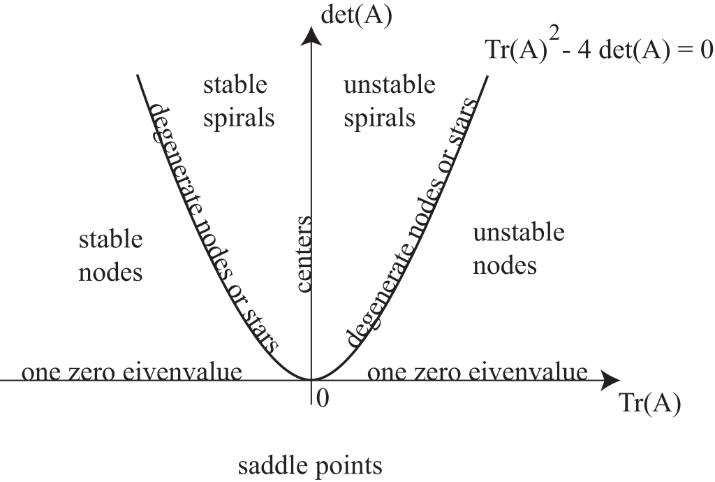
The fixed point [latex]Y = Y_0[/latex] of (13.4) is linearly stable if all solutions of the linearized system (13.5) converge towards the origin as [latex]t \rightarrow + \infty[/latex]. This only occurs if the real parts of [latex]\lambda_1[/latex] and [latex]\lambda_2[/latex] are both negative, which implies that the trace of [latex]A[/latex] is also negative. If we assume that [latex]F[/latex] is real, as we do from now on, then [latex]A[/latex] has real coefficients and its eigenvalues are either both real or complex conjugate of one another. In this case, a linearly stable fixed point is such that both [latex]\text{Tr} (A) = \lambda_1 + \lambda_2 < 0[/latex] and [latex]\det (A) = \lambda_1 \lambda_2 > 0[/latex].

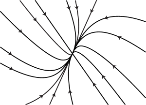
If the eigenvalues of [latex]A[/latex] are both negative, real and distinct, then the fixed point is a stable node. The phase portrait of the linear system (13.5) looks like the sketch of Figure 13.1. Note that the trajectories are tangent at the origin to the eigendirection associated with the slowest eigenvalue.

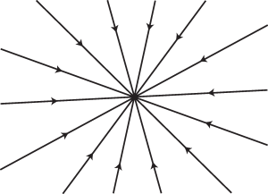
If [latex]A[/latex] is proportional to the identity matrix (i.e. if the eigenvalues of [latex]A[/latex] are the same but the corresponding eigenspace is two-dimensional), then the fixed point [latex]Y=Y_0[/latex] is called a star.

If the eigenvalues of [latex]A[/latex] are the same but the corresponding eigenspace is one-dimensional, then [latex]Y=Y_0[/latex] is called a degenerate node.

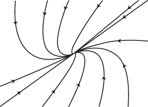
Figures 13.2 and 13.3 show the typical phase portrait of the linear system (13.5) when the fixed point is a stable star and a stable degenerate node, respectively.

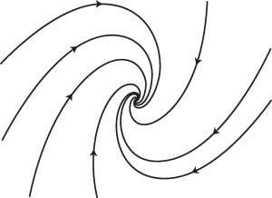
If the eigenvalues of [latex]A[/latex] have non-zero imaginary parts, then [latex]Y=Y_0[/latex] is a stable spiral. The corresponding phase portrait of (13.5) is shown in Figure 13.4.

If one of the eigenvalues of [latex]A[/latex] has positive real part, then the fixed point [latex]Y=Y_0[/latex] is linearly unstable. This occurs if either [latex]\det(A)<0[/latex], in which case the fixed point is a <em>saddle point, or if [latex]\det(A)>0[/latex] and [latex]\text{Tr} (A) > 0[/latex].

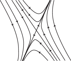
The phase portrait of (13.5) when the origin is a saddle point is shown in Figure 13.5. The phase portraits of (13.5) when the origin is an unstable node, an unstable star, an unstable degenerate node, or unstable spiral are similar to those of Figures 13.1, 13.2, 13.3, and 13.4, but with the direction of the arrows reversed.

If [latex]\det(A)=0[/latex] and [latex]\text{Tr} (A) \ne 0[/latex], then one of the eigenvalues of [latex]A[/latex] is zero, and system (13.5) has a line of fixed points.

This is a degenerate situation and in most cases the dynamical system (13.4) has a single fixed point, even though its linearization has a continuous family of fixed points. The phase portrait of (13.5) in a case where [latex]\lambda_1 < 0[/latex] and [latex]\lambda_2 = 0[/latex] is shown in Figure 13.6.

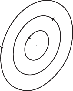
Finally, if all of the eigenvalues of [latex]A[/latex] have zero real part, then [latex]Y=Y_0[/latex] is marginally stable. Since we ignore the non-generic situation where [latex]A = 0[/latex], this implies that [latex]A[/latex] has purely imaginary complex conjugate eigenvalues, and the fixed point [latex]Y=Y_0[/latex] is called a linear center. In this case, [latex]\det(A) > 0[/latex] but [latex]\text{Tr} (A) = 0[/latex]. Figure 13.7 shows the phase portrait of the linear system (13.5) when the origin is a (linear) center. Determining whether the fixed point [latex]Y = Y_0[/latex] is a nonlinear center for the dynamical system (13.4) requires further analysis.

The above results can be summarized in the diagram of Figure 13.8, which shows the classification of the fixed point [latex]X = 0[/latex] of the linear system (13.5), as a function of the trace and determinant of [latex]A[/latex].

The Hartman-Grobman theorem indicates that for a smooth dynamical system, the nature of a fixed point is not changed by nonlinear terms provided the fixed point is hyperbolic, i.e. provided the eigenvalues of the Jacobian of its linearization all have non-zero real parts. Linear stability analysis can therefore be used to classify hyperbolic fixed points of nonlinear dynamical systems. Further analysis is required to determine the nonlinear stability of non-hyperbolic fixed points. In particular, centers may remain centers or become stable or unstable spirals. Methods to investigate the effect of nonlinearities on hyperbolic and non-hyperbolic fixed points are typically discussed in an introductory text on dynamical systems.