The law of mass action

Consider a chemical reaction

[latex]\begin{array}{ccc} & k & \\ A + B &\rightarrow& C, \end{array}[/latex]

where [latex]A[/latex], [latex]B[/latex] and [latex]C[/latex] represent chemicals, [latex]A[/latex] and [latex]B[/latex] are the reactants, [latex]C[/latex] is the product, and [latex]k > 0[/latex] is the rate constant of the reaction. The law of mass action describes how the concentrations of [latex]A[/latex], [latex]B[/latex] and [latex]C[/latex] change as a consequence of this reaction. The idea is that the reaction will take place if chemicals [latex]A[/latex] and [latex]B[/latex] collide, and if their energy is higher than the energy of activation of the reaction. The number of successful (i.e. leading to a reaction) collisions between [latex]A[/latex] and [latex]B[/latex] is proportional to the product of the concentrations of [latex]A[/latex] and [latex]B.[/latex] The constant of proportionality is the constant [latex]k[/latex]. We thus write the following differential equations for the expected values of [latex][A][/latex], [latex][B][/latex], [latex][C][/latex], (recall that we are in a situation where large numbers of molecules of reactants and products are present)

[latex]\displaystyle \frac{d [A]}{d t} = \frac{d [B]}{d t} = - k [A]\,[B] = - \frac{d [C]}{d t},[/latex]

where [latex][I][/latex] denotes the concentration of chemical [latex]I[/latex]. If [latex]A = B[/latex], so that the chemical reaction is

[latex]\begin{array}{ccc} & k & \\ 2 A &\rightarrow& C, \end{array}[/latex]

we need two molecules of [latex]A[/latex] to create one product molecule [latex]C[/latex], leading to

[latex]\displaystyle \frac{1}{2} \frac{d [A]}{d t} = - k [A]^2 = - \frac{d [C]}{d t}.[/latex]

If a reaction is reversible, for instance if

[latex]\begin{array}{ccc} & k_1 & \\ A + B & \rightleftharpoons & C, \\ & k_2 & \end{array}[/latex]

then [latex]A[/latex] is consumed at relative rate [latex]k_1[/latex] and produced at relative rate [latex]k_2[/latex], so that

[latex]\displaystyle \frac{d [A]}{d t} = - k_1 [A]\, [B] + k_2 [C],[/latex]

and similarly for [latex][B][/latex] and [latex][C][/latex].

Finally, if a reaction process involves more than one chemical reaction, the rates of change of a chemical due to each of the reactions are added up in order to obtain the global rate of change of that chemical. For instance, assume that we have a system described by

[latex]\begin{array}{ccc} & k_1 & \\ A + B & \rightleftharpoons & C, \\ & k_2 & \end{array}[/latex]

[latex]\begin{array}{ccc} & k_3 & \\ C + A &\rightarrow & D. \end{array}[/latex]

Then the concentration of [latex]A[/latex] evolves according to

[latex]\displaystyle \frac{d [A]}{d t} = - k_1 [A]\,[B] + k_2 [C] - k_3 [C]\,[A],[/latex]

and the rate equations for [latex]B[/latex], [latex]C[/latex] and [latex]D[/latex] are

[latex]\displaystyle \frac{d [B]}{d t} = - k_1 [A]\,[B] + k_2 [C],[/latex]

[latex]\displaystyle \frac{d [C]}{d t} = k_1 [A]\,[B] - k_2 [C] - k_3 [C]\,[A],[/latex]

[latex]\displaystyle \frac{d [D]}{d t} = k_3 [C]\,[A].[/latex]

Note that the net reaction associated with this process is [latex]2 A + B \rightarrow D[/latex]. The rate equations must be written for each of the steps involved in the reaction, and not on the basis of the net reaction.

Chemical reactions can thus be described in terms of coupled nonlinear ordinary differential equations, and the theory of dynamical systems therefore applies to their analysis.

The Brusselator and Oregonator models

Because rate equations describing chemical oscillations are nonlinear, it is possible to observe reactions which are oscillatory in time, in the same way as the Lotka-Volterra equations may describe oscillations in a predator-prey system. The Belousov-Zhabotinsky reaction is the classical example of an oscillatory chemical reaction. When Russian biochemist Boris P. Belousov^[1] reported his findings in 1951, his results were initially received with disbelief. It is only after A.M. Zhabotinsky^[2] reproduced and improved Belousov’s experiments, that the existence of oscillatory reactions was finally accepted. There are two classical models for oscillatory reactions, called the “Brusselator” (proposed by a group in Brussels^[3]) and the “Oregonator” (proposed by chemists at the University of Oregon^[4]). We briefly discuss each of them below.

The Brusselator

Consider the following hypothetical chemical process (Glansdorff & Prigogine, 1971).

[latex]\begin{array}{ccc} & k_1 & \\ A &\rightarrow& X, \end{array}[/latex]

[latex]\begin{array}{ccc} & k_2 & \\ 2 X + Y &\rightarrow& 3 X, \end{array}[/latex]

[latex]\begin{array}{ccc} & k_3 & \\ B + X &\rightarrow& Y + D, \end{array}[/latex]

[latex]\begin{array}{ccc} & k_4 & \\ X &\rightarrow& E, \end{array}[/latex]

where the rate constants [latex]k_i[/latex] are all equal to 1. The corresponding rate equations for [latex][X][/latex] and [latex][Y][/latex] form the Brusselator model, which reads

[latex]\displaystyle \left\{\begin{align} \displaystyle \frac{d [X]}{d t} & = [A] + [X]^2\,[Y] - [B]\,[X] - [X],\\ \displaystyle \frac{d [Y]}{d t} & = - [Y]\,[X]^2 + [B]\,[X], \end{align}\right. \qquad (8.1)[/latex]

where [latex][A][/latex] and [latex][B][/latex] are parameters. It has a unique fixed point [latex]P[/latex], given by [latex][X]=[A][/latex] and [latex][Y]=[B]/[A][/latex]. From a dimensional analysis point of view, these expressions may look strange, but we lost track of the dimensions when we set all of the reaction constants (which had different dimensions) to unity (see exercises).

The Jacobian of (8.1) about the fixed point [latex]P[/latex] is

[latex]J(P) = \left(\begin{array}{cc} [B] - 1 & [A]^2 \\ -[B] & -[A]^2 \end{array}\right),[/latex]

and its determinant is equal to [latex][A]^2 > 0[/latex]. The stability of the fixed point therefore depends on the sign of the trace of [latex]J(P)[/latex], which is equal to [latex]T = [B]-1-[A]^2[/latex]. It is easy to see that if [latex][X][/latex] or [latex][Y][/latex] are sufficiently large, then [latex]{d[Y]} / {d[X]} \simeq -1,[/latex] and trajectories are almost straight lines with slope -1. However, as [latex][Y][/latex] gets close to 0, these trajectories cannot leave the first quadrant, since [latex]d[Y]/d t \gt 0[/latex] if [latex][Y]=0[/latex] and [latex][X] \gt 0[/latex]. Since at that time we also have [latex]d[X]/dt \lt 0[/latex] if [latex][X][/latex] is large enough, we expect the trajectories to be brought back towards regions where both [latex][X][/latex] and [latex][Y][/latex] are of order one.

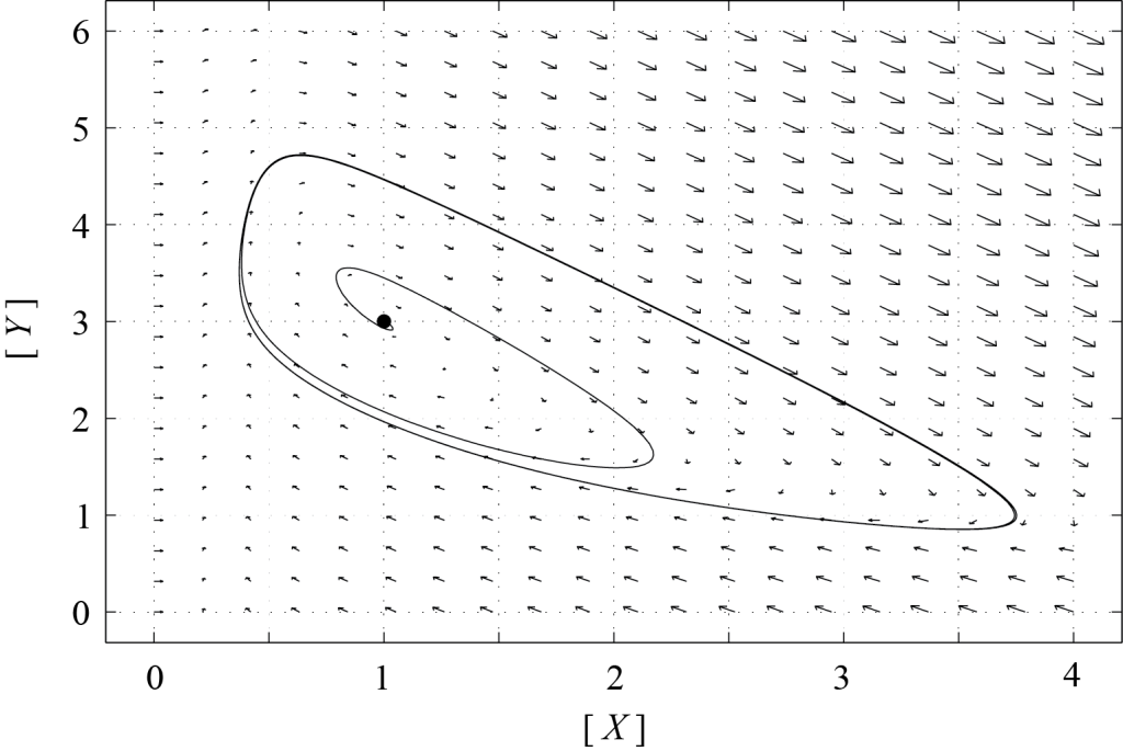
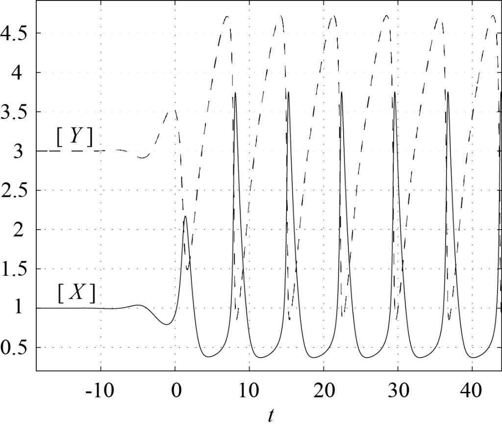
If [latex]P[/latex] is stable, i.e. if [latex]T \lt 0[/latex], then all trajectories should end up at [latex]P[/latex]. However, if [latex]P[/latex] is an unstable node or an unstable spiral, trajectories cannot converge towards [latex]P[/latex], and there must be another attractor of the dynamics. Figure 8.1 shows the phase portrait of (8.1) with [latex][A]=1[/latex] and [latex][B]=3[/latex] (so that [latex]T = 1 > 0[/latex]). The second attractor is a limit cycle, towards which all trajectories converge. Only one trajectory is plotted in this figure. The corresponding plots of [latex][X][/latex] and [latex][Y][/latex] as functions of time are shown in Figure 8.2. One can see that on the limit cycle, [latex][X][/latex] remains small most of the time, then quickly increases to a maximum value and comes back towards zero, in a periodic fashion. As [latex][X][/latex] increases, [latex][Y][/latex] drops abruptly, and then slowly grows back to its maximum value while [latex][X][/latex] remains small. Such relaxation oscillations are typical of many oscillatory chemical reactions.

The Oregonator

The Oregonator was proposed by R.J. Fields and R.M. Noyes in 1974. It corresponds to the following chemical reactions

[latex]\begin{array}{ccc} & k_1 & \\ A + Y &\rightarrow& X, \end{array}[/latex]

[latex]\begin{array}{ccc} & k_2 & \\ X + Y &\rightarrow& P, \end{array}[/latex]

[latex]\begin{array}{ccc} & k_3 & \\ B + X &\rightarrow& 2 X + Z, \end{array}[/latex]

[latex]\begin{array}{ccc} & k_4 & \\ 2 X &\rightarrow& Q, \end{array}[/latex]

[latex]\begin{array}{ccc} & k_5 & \\ Z &\rightarrow& f Y, \end{array}[/latex]

where [latex][A][/latex] and [latex][B][/latex] are constant, and [latex]f[/latex] is a stoichiometric factor. The corresponding rate equations are

[latex]\displaystyle \left\{\begin{align} \displaystyle \frac{d [X]}{d t} & = k_1 [A]\, [Y] - k_2 [X]\,[Y] + k_3 [B]\,[X] - 2 k_4 [X]^2,\\ \displaystyle \frac{d [Y]}{d t} & = - k_1 [A]\, [Y] - k_2 [X]\,[Y] + k_5 f [Z], \\ \displaystyle \frac{d [Z]}{d t} & = k_3 [B] \, [X] - k_5 [Z]. \end{align}\right.[/latex]

Field and Noyes (1974) defined the following dimensionless quantities

[latex]x = \displaystyle \frac{[X]}{X_0},\qquad y = \displaystyle \frac{[Y]}{Y_0},\qquad z = \displaystyle \frac{[Z]}{Z_0},\qquad \tau = \displaystyle \frac{t}{T_0},[/latex]

where

[latex]X_0 = \displaystyle \frac{k_1}{k_2} [A],\quad Y_0 = \displaystyle \frac{k_3}{k_2} [B], \quad Z_0 = \displaystyle \frac{k_1 k_3}{k_2 k_5} [A] [B], \quad \displaystyle T_0 = \frac{1}{\sqrt{k_1 k_3 [A] [B]}}.[/latex]

Then, the dimensionless form of the Oregonator becomes

[latex]\displaystyle \left\{\begin{align} \displaystyle \frac{d x}{d \tau} & = s (y - x y + x - q x^2),\\ \displaystyle \frac{d y}{d \tau} & = \frac{1}{s} (- y - x y + f z), \\ \displaystyle \frac{d z}{d \tau} & = \omega (x - z), \end{align}\right. \qquad (8.2)[/latex]

where

[latex]s = \displaystyle \sqrt{\frac{k_3 [B]}{k_1 [A]}}, \qquad q = \displaystyle \frac{2 k_1 k_4 [A]}{k_2 k_3 [B]}, \qquad \omega = \displaystyle \frac{k_5}{\sqrt{k_1 k_3 [A] [B]}}.[/latex]

By assuming that [latex]x[/latex] quickly reaches a steady-state value, it is possible to reduce Equations (8.2) to a two-dimensional dynamical system. Indeed, setting [latex]d x / d \tau = 0[/latex] gives

[latex]x = \displaystyle \frac{1}{2 q} \left(1 - y + \sqrt{(1 - y)^2 + 4 q y}\right),[/latex]

and by substituting this expression into (8.2), one obtains

[latex]\displaystyle \left\{\begin{align} \displaystyle \frac{d y}{d \tau} & = \frac{1}{s} \left(- y - \frac{y}{2 q} \left(1 - y + \sqrt{(1 - y)^2 + 4 q y}\right) + f z \right), \\ \displaystyle \frac{d z}{d \tau} & = \omega \left(\frac{1}{2 q} \left(1 - y + \sqrt{(1 - y)^2 + 4 q y}\right) - z \right). \end{align}\right. \qquad (8.3)[/latex]

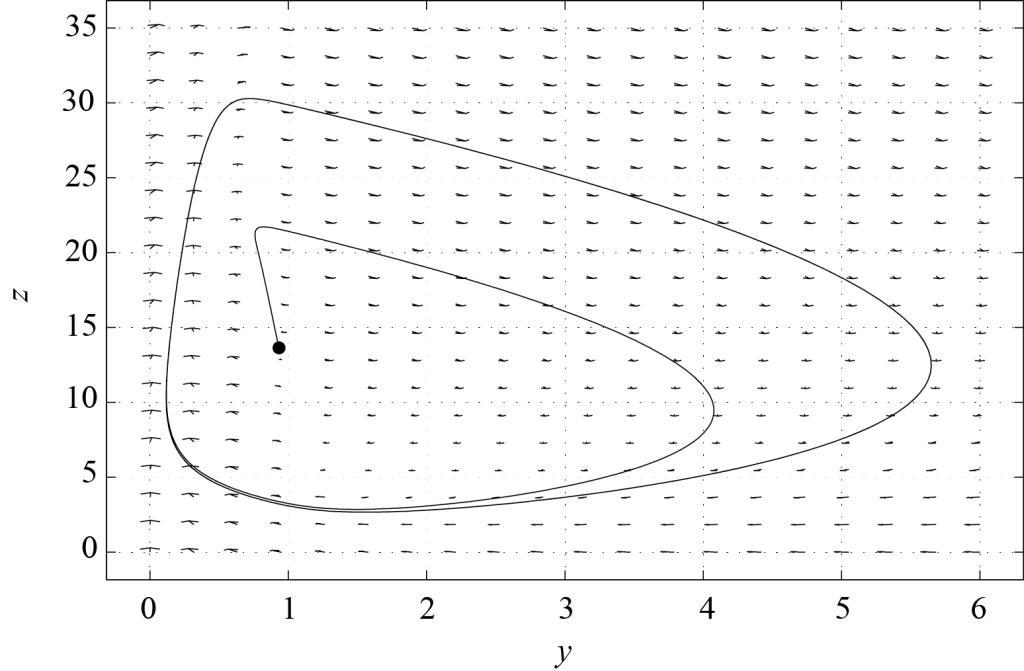
In what follows, we set [latex]f = 1[/latex]. Field and Noyes (1974) estimated the values of [latex]s[/latex], [latex]q[/latex], [latex]\omega[/latex] as well as of all dimensionless variables for the Belousov-Zhabotinsky reaction. Details can be found in their article entitled Oscillations in chemical systems. IV. Limit cycle behavior in a model of a real chemical reaction. They also concluded that the Oregonator model is capable of predicting oscillations for the concentrations of the chemicals involved in the reaction process. Realistic parameters make the problem very stiff (i.e. there are both very short and very long characteristic time scales, which is typical for excitable systems), but model (8.3) also exhibits oscillations in reasonably stiff cases. Figure 8.3 shows the phase plane of model (8.3) with parameters [latex]s = 1[/latex], [latex]q = 0.01[/latex], and [latex]\omega = 2[/latex]. Trajectories starting from the fixed point with both [latex]y[/latex] and [latex]z[/latex] non-zero converge towards a limit cycle. As a consequence, the variables [latex]y[/latex] and [latex]z[/latex] oscillate in time, and so do [latex][X][/latex], [latex][Y][/latex] and [latex][Z][/latex] in the Oregonator model.

Chemical waves

When a chemical reaction takes place in a spatially extended system, diffusion should be taken into account. As a consequence, the rate equations discussed above are turned into partial differential equations. The reaction terms remain the same, but the concentration of each chemical now diffuses with a diffusion coefficient which depends on the size and weight of the molecule in question. If the reaction is oscillatory, wave fronts, corresponding to say large concentrations of some chemical, propagate in the system. Moreover, if the reaction is constrained to a two-dimensional surface and the wave is initiated at some point in space, then the wave fronts are circular. As an example, a 2001 article by C. Sachs  et al.^[5] describes how such wave fronts are observed in an experiment, and proposes a reaction-diffusion model which reproduces this behavior. The authors also discuss the limitation of reaction-diffusion models when macroscopic parameters are affected by the details of microscopic interactions.

What would happen if the wave front was broken, for instance if the wave went over a region where the reaction could not take place? If the wave front is anchored at one point, then it will curve and eventually form a spiral wave. Such waves are often observed in experiments where the Belousov-Zhabotinsky reaction is constrained to a two-dimensional surface, such as a thin film, a porous glass disk, or even a sheet of filter paper. The article by S.C. Müller et al.^[6] discusses experiments revealing the structure of the core of such spiral waves.

Summary

We started with the law of mass action, which allowed us to describe the dynamics of the (average) concentrations of reactants and products involved in chemical reactions. In particular, we considered two hypothetical sets of chemical reactions called the Brusselator and the Oregonator. By applying the methods of analysis discussed in the previous chapters, we concluded that it was possible for these chemical systems to exhibit oscillatory dynamics. This provides a proof of concept for oscillatory reactions such as the Belousov-Zhabotinsky reaction. In spatially extended systems, the latter leads to chemical waves and spiral defects, whose structure is well documented in the research literature.