Viral infections

We first model the dynamics of a viral infection, such as hepatitis B or C, and are interested in describing how the corresponding virus can spread and multiply in a person’s body. Denote by [latex]X[/latex] the average number of uninfected cells, which virions will try to infect; let [latex]Y[/latex] be the average number of infected cells, and [latex]V[/latex] be the average viral load (or the number of free virions in the body). Consider that uninfected cells are produced at a constant rate [latex]\lambda[/latex] by the body, die at rate [latex]\delta X[/latex], and become infected at rate [latex]f(X,V) X[/latex], where [latex]f[/latex] is some function of [latex]X[/latex] and [latex]V[/latex]. As a consequence, infected cells [latex]Y[/latex] are created at rate [latex]f(X,V) X[/latex], and we assume they die at rate [latex]a Y[/latex]. Finally, free virions are produced at a rate proportional to the number of infected cells [latex]k Y[/latex], and are removed or destroyed at rate [latex]\kappa V[/latex]. If we consider that, as a first approximation, [latex]f[/latex] is a linear function of [latex]V[/latex], i.e. [latex]f(X,V) = b V[/latex], we have the following model.^[1]

[latex]\left\{\begin{align} \displaystyle \frac{d X}{d t} & =\lambda - \delta X - b V X, \\ \displaystyle \frac{d Y}{d t} & = b V X - a Y,\\ \displaystyle \frac{d V}{d t} & = k Y - \kappa V, \end{align}\right. \qquad (7.1)[/latex]

This model has six parameters and four variables. We can rescale time and [latex]V[/latex], but it is not a good idea to rescale [latex]X[/latex] and [latex]Y[/latex] independently since they both count cells and the term in [latex]b V X[/latex] transfers cells from the [latex]X[/latex] compartment to the [latex]Y[/latex] compartment. We can therefore reduce Equations (7.1) to a model with three parameters. More precisely, let

[latex]\tau = \delta t, \qquad \displaystyle x = \frac{k b}{\delta^2} X, \qquad y = \frac{k b}{\delta^2} Y, \qquad v = \frac{b}{\delta} V.[/latex]

Then, the scaled version of Equations (7.1) is

[latex]\left\{\begin{align} \displaystyle \frac{d x}{d \tau} & = \zeta - x - v\, x,\\ \displaystyle \frac{d y}{d \tau} & = v\, x - \eta\, y,\\ \displaystyle \frac{d v}{d \tau} & = y - \mu\, v, \end{align}\right. \qquad (7.2)[/latex]

where [latex]\zeta = \displaystyle \frac{\lambda k b}{\delta^3},[/latex] [latex]\eta = \displaystyle \frac{a}{\delta},[/latex] and [latex]\mu = \displaystyle \frac{\kappa}{\delta}[/latex] are dimensionless parameters.

We scaled time according to the death rate of normal cells. Alternatively, we could have scaled time according to the rate at which normal cells are produced by the body, i.e. we could have defined [latex]\tau = \lambda t / X_0[/latex], with [latex]X_0 = \delta^2 / (k b)[/latex]. We could also have used a combination of these two time scales. In general, there is more than one possible way of defining dimensionless variables. The most convenient choice is often that which gives dimensionless parameters of order one, if at all possible.

We refer the reader to the 1998 article by A.U. Neumann et al., entitled Hepatitis C viral dynamics in vivo and the antiviral efficacy of interferon-alpha therapy, to see how estimating parameters in model (7.1) may be used to understand the role of interferons in hepatitis C therapy.

Modeling infectious diseases

There is ample literature on the modeling of infectious diseases (for a review, see for instance the 2000 article by H. Hethcote, entitled The Mathematics of Infectious Diseases). The most general basic model is called the MSEIRS model. Each letter in the acronym refers to a particular class or compartment of the population, and the ordering of the letters is such that individuals belonging to one class move to the class on the right under the effect of the disease. The various classes are defined as follows.

• Class M corresponds to infants with passive immunity. Typically, these are newborns whose mothers were infected, and who received antibodies through the placenta before birth.
• Class S is the class of susceptible individuals, who may become infected by the disease. Infants in class M have temporary immunity and eventually move to class S.
• Class E corresponds to exposed individuals, who have been in contact with an infected person.
• Class I is the class of infectious individuals, who can transmit the disease.
• Class R corresponds to individuals who have recovered (or died) from the disease, or who have been removed from the group of people affected by the disease.

Depending on the type of infectious disease, individuals in class R may have acquired permanent immunity. In this case, the appropriate model is of the MSEIR type. However, if individuals in class R eventually become susceptible again, then an MSEIRS model should be used. Most realistic models couple the classes described above with age groups. Some models consider the age [latex]a[/latex] of a person as an independent variable. Other classes, such as symptomatic and asymptomatic groups of individuals, may be considered, and the appropriate number of compartments, as well as their nature, is selected by the modeler. Applications of compartmental models include disease forecasting, as well as predicting the effectiveness of vaccination or of a disease eradication campaign. Below, we only discuss two simple models, namely the classic and endemic SIR models.

The SIR model

The classic SIR model does not include classes M and E, and reads

[latex]\left\{\begin{align} \displaystyle \frac{d S}{d t} & = - \alpha S \frac{I}{N},\\ \displaystyle \frac{d I}{d t} & = \alpha S \frac{I}{N} - \beta I,\\ \displaystyle \frac{d R}{d t} & = \beta I, \end{align}\right. \qquad (7.3)[/latex]

with initial conditions [latex]S(0) = S_0 \ge 0,[/latex] [latex]I(0)=I_0 \gt 0,[/latex] and [latex]R(0) \ge 0.[/latex] Here, [latex]S[/latex], [latex]I[/latex] and [latex]R[/latex] are the expected numbers of individuals in each compartment, and [latex]N = S + I + R[/latex] is the total population. Note that births and deaths are not included in the model. This typically works for diseases which evolve over a short period of time, so that changes in the total population are negligible.

In this model, [latex]I/N[/latex] represents the fraction of infectious individuals. The product of this quantity with the contact rate [latex]\alpha > 0[/latex] measures the average number of positive (i.e. giving rise to transmission of the disease) contacts per susceptible individual per unit of time. Since there are on average [latex]S[/latex] susceptible individuals, the rate of change of [latex]S[/latex] is [latex]- \alpha S I /N[/latex]. The number of infected individuals increases by contact with susceptibles, and decreases due to recovery, at rate [latex]- \beta I[/latex], with [latex]\beta \ge 0[/latex]. By adding up the three equations, one easily checks that [latex]d N / d t = 0[/latex], as expected since we neglected births and deaths. System (7.3) can thus be reduced to a two-dimensional system of ordinary differential equations, by omitting the last equation for [latex]R[/latex]. The remaining two equations may be written in dimensionless form by letting

[latex]s = \displaystyle \frac{S}{N},[/latex] [latex]i = \displaystyle \frac{I}{N},[/latex] and [latex]\tau = \alpha t.[/latex]

Then, the first two equations of (7.3) become

[latex]\left\{\begin{align} \displaystyle \frac{d s}{d \tau} & =- s i,\\ \displaystyle \frac{d i}{d \tau} & = s i - \delta i, \end{align}\right. \qquad (7.4)[/latex]

where [latex]\delta = \beta / \alpha > 0[/latex]. The quantity [latex]\sigma = 1 /\delta[/latex] is the contact rate [latex]\alpha[/latex] multiplied by the characteristic time [latex]1 / \beta[/latex] during which a person remains infectious. It is called the contact number of the disease, and in this case is equal to the basic reproduction number  [latex]R_0[/latex] of the infection described by the SIR model.

Since [latex](1 - s - i) N = R \ge 0[/latex], Equations (7.4) only make biological sense if [latex]s[/latex] and [latex]i[/latex] remain positive and such that [latex]s + i \le 1[/latex], provided initial conditions satisfy these requirements. In other words, trajectories of the dynamical system (7.4) that start in the triangle

[latex]{\mathcal T} = \left\{ (s,i) | s \ge 0,\ i \ge 0,\ s + i \le 1\right\}[/latex]

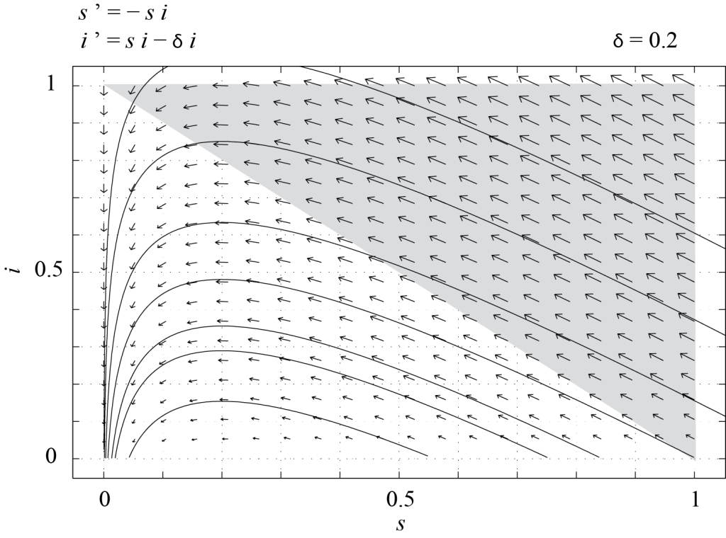
should remain in [latex]\mathcal T.[/latex] To check this, consider the dynamics on the boundary of [latex]\mathcal T.[/latex] First assume that [latex]s = 0[/latex] and [latex]i \le 1[/latex]. Then [latex]d s / d \tau = 0[/latex], i.e. [latex]s[/latex] remains equal to zero, and [latex]i[/latex] decreases towards zero, but does not become negative. Similarly, if [latex]i = 0[/latex], then both [latex]s[/latex] and [latex]i[/latex] remain constant (what is the biological significance of this fact?). Finally, if [latex]s + i = 1[/latex], then [latex]\displaystyle \frac{d}{d \tau} (s + i) = - \delta i \le 0,[/latex] so that [latex]s+i[/latex] will not increase past the value 1. System (7.4) has an infinite number of fixed points in [latex]{\mathcal T}[/latex], which are such that [latex]i = 0[/latex] and [latex]s[/latex] is arbitrary.

Figure 7.1 shows the phase portrait of (7.4), obtained with PPLANE, with [latex]\delta = 0.2[/latex]. In this case, we see that all trajectories in [latex]\mathcal T[/latex] converge towards one of the fixed points, i.e. [latex]\displaystyle \lim_{t \rightarrow \infty} i = 0.[/latex] This means that the epidemic eventually dies out, and we are only left with susceptible individuals and/or those who have recovered from the disease.

The classic endemic model

For an endemic disease, births and deaths need to be taken into account, and the SIR model becomes

[latex]\left\{\begin{align} \displaystyle \frac{d S}{d t} & = \nu N - \mu S- \alpha S \frac{I}{N},\\ \displaystyle \frac{d I}{d t} & = - \mu I +\alpha S \frac{I}{N} - \beta I,\\ \displaystyle \frac{d R}{d t} & = - \mu R + \beta I, \end{align}\right. \qquad (7.5)[/latex]

with initial conditions [latex]S(0) = S_0 \ge 0,[/latex] [latex]I(0)=I_0 \gt 0,[/latex] and [latex]R(0) \ge 0.[/latex] Here the new parameters are the per capita death rate [latex]\mu[/latex] and per capita birth rate [latex]\nu[/latex] of the population. By choosing [latex]\mu = \nu[/latex], the total population [latex]N = S + I + R[/latex] is constant. In this case, using the same dimensionless variables as for the classic SIR model, we are left with a two-dimensional dynamical system, which reads, in dimensionless form,

[latex]\left\{\begin{align} \displaystyle \frac{d s}{d \tau} & = \eta - \eta s - s i,\\ \displaystyle \frac{d i}{d \tau} & = - (\eta+\delta) i + s i, \end{align}\right. \qquad (7.6)[/latex]

where [latex]\eta = \nu / \alpha = \mu /\alpha[/latex].

As before, it is easy to check that trajectories starting in [latex]\mathcal T[/latex] remain in [latex]\mathcal T[/latex] (see exercises). The fixed points of (7.6) in the [latex](s,i)[/latex] plane are

[latex]P_1 = (1, 0) \qquad \text{and} \qquad P_2 = \left(\eta + \delta, \displaystyle \frac{\eta (1 - \eta - \delta)}{\eta + \delta}\right).[/latex]

The Jacobian of (7.6) is

[latex]J(s,i) = \left(\begin{array}{cc} - \eta - i & - s \\ i & s - (\eta + \delta) \end{array} \right)[/latex]

and

[latex]J(P_1) = \left(\begin{array}{cc} - \eta & - 1 \\ 0 & 1 - (\eta + \delta) \end{array} \right).[/latex]

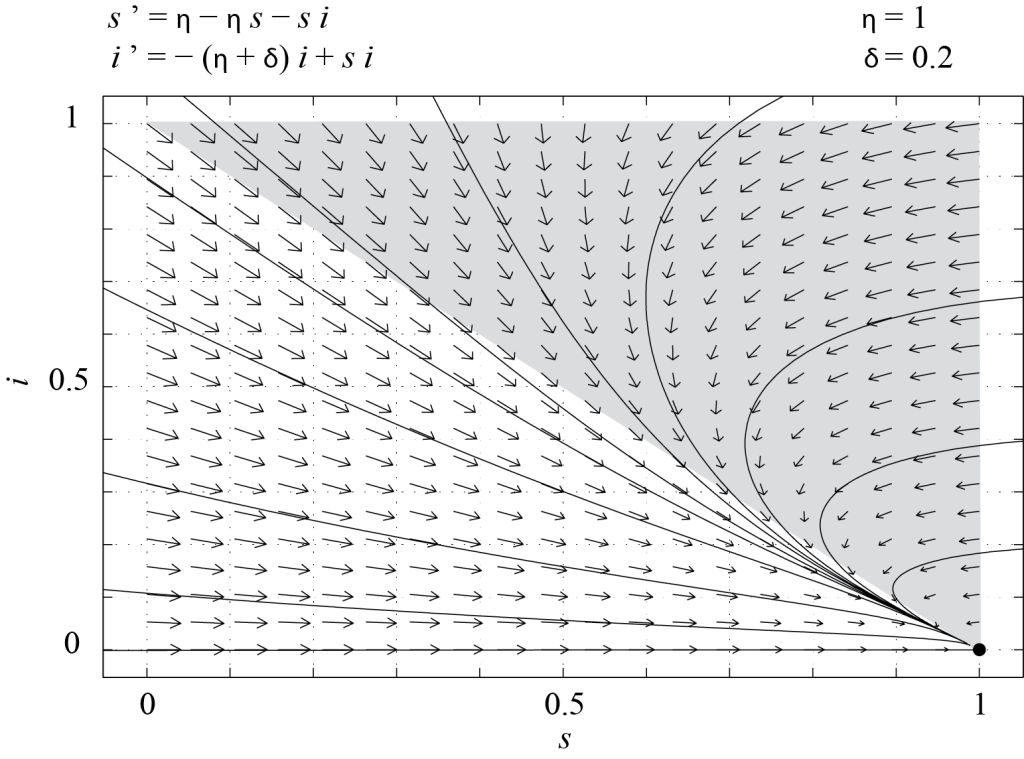
Whether [latex]P_2[/latex] is in [latex]\mathcal T[/latex] depends on the parameters [latex]\delta[/latex] and [latex]\eta[/latex]. More precisely, [latex]P_2 \in {\mathcal T} \Leftrightarrow 0 \lt \eta + \delta \le 1.[/latex] Therefore, if [latex]\eta + \delta > 1[/latex], [latex]P_1[/latex] is the only fixed point in [latex]\mathcal T[/latex] and since the eigenvalues of [latex]J(P_1)[/latex] are [latex]-\eta[/latex] and [latex]1 - (\eta + \delta)[/latex], [latex]P_1[/latex] is a stable node. All of the trajectories starting in [latex]\mathcal T[/latex] must converge to this fixed point, which means that in the long run there are only susceptible individuals in the population. This is because those who have recovered from the disease eventually die and are replaced by newborns, who are susceptible. This is illustrated in Figure 7.2, which shows the phase portrait of (7.6), obtained with PPLANE, with [latex]\delta = 0.2[/latex] and [latex]\eta = 1[/latex].

If on the other hand [latex]\eta + \delta \lt 1[/latex], then [latex]P_1[/latex] is a saddle, and

[latex]J(P_2) = \left(\begin{array}{cc} -\displaystyle \frac{\eta}{\eta+\delta} & -(\eta + \delta) \\ \displaystyle \frac{\eta (1 - \eta - \delta)}{\eta + \delta} & 0 \end{array} \right).[/latex]

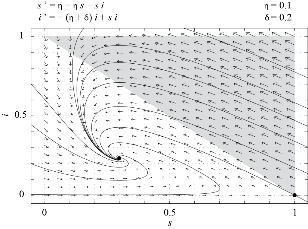
The determinant of [latex]J(P_2)[/latex] is equal to [latex]\eta (1 - \eta - \delta)[/latex] and is positive. The trace of [latex]J(P_2)[/latex] is negative, so [latex]P_2[/latex] is either a stable spiral or a stable node. Trajectories starting in [latex]\mathcal T[/latex] converge to [latex]P_2[/latex], which is called the endemic equilibrium. In this case, the disease is always present in the population and there is always a non-zero number of infected individuals. Figure 7.3 shows the phase portrait of (7.6) with [latex]\eta = 0.2[/latex] and [latex]\delta=0.1[/latex].

Summary

This chapter illustrates how the modeling concepts discussed in the previous chapters may be applied to the description, in terms of ordinary differential equations, of the dynamics of infectious diseases and the spread of epidemics. Moreover, it provides the reader with a basic introduction to the terminology and applications of compartmental models.

It should be clear by now that models of arbitrary complexity may be built from the simple tools discussed in this text. The modeling process is always the same, no matter how involved the model is. The methods of analysis, in terms of maps or differential equations, are also similar, but become more complicated as the dimension of the model is increased. In particular, three-dimensional continuously differentiable dynamical systems may exhibit chaos, the understanding of which requires more advanced techniques than those discussed here. The section on further reading includes texts on dynamical systems and chaos that the reader may want to consult.