Pattern Formation

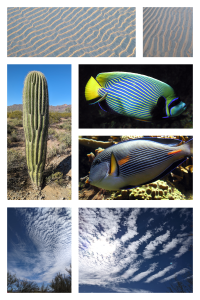
Patterns (see Figure 10.1), such as stripes and spots on animal coats or sand ripples on a beach, are very common in nature and in carefully controlled laboratory experiments. They typically occur in systems which are driven far from equilibrium by external forces or sources of energy. When the forcing is larger than what is necessary to balance inertial forces, the system responds by reorganizing itself into a periodic structure, called a pattern. There are many types of patterns, such as rolls, squares or hexagons, and they can be stationary or dynamic. The study of pattern-forming systems has been the subject of active research in physics, chemistry, nonlinear optics and applied mathematics for more than half a century^[1]. In what follows, we will briefly mention Turing patterns, explore a canonical pattern-forming model, known as the complex Swift-Hohenberg equation, and discuss a reaction-diffusion model for vegetation patterns.

Turing patterns

In 1952, A.M. Turing^[2] proposed the idea that differentiation patterns such as those selecting regions where a hydra grows its tentacles, were in fact chemical patterns, in particular those corresponding to stationary periodic structures^[3]. Turing explained how such patterns could result from the instability of a homogeneous solution to a set of coupled reaction-diffusion equations. This instability was described as a symmetry-breaking instability, since the periodic structure that grew as a result of the instability broke the translational invariance of the initial homogeneous solution. It is only in the 1990s that Turing patterns were seen in chemical experiments^[4][5], in the form of hexagons and stripes, but also as irregular structures corresponding to a state of chemical turbulence^[6].

The complex Swift-Hohenberg equation

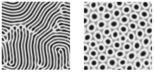
We will explore pattern formation by means of a single model, called the complex Swift-Hohenberg equation. Depending on whether the parameters of this model are real or complex, stationary or traveling patterns will be observed. Figure 10.2 shows stripe and hexagon patterns produced by this model. The general theory of pattern formation^[7] explains why different models may produce patterns that are similar, and as a consequence why different chemical, physical or biological systems may display patterns that look alike. It also justifies the use of a generic pattern forming model to understand the mechanisms involved in pattern formation, as we do in the next section.

Consider the following partial differential equation

[latex]\displaystyle \frac{\partial \psi}{\partial t} = (\mu + i \nu) \psi - (\alpha + i \beta) \left(\Omega + \frac{\partial^2}{\partial x^2} + \frac{\partial^2}{\partial y^2}\right)^2 \psi + i \eta \left(\frac{\partial^2}{\partial x^2} + \frac{\partial^2}{\partial y^2}\right) \psi - (\gamma + i \delta) |\psi|^2 \psi - \zeta |\psi|^2, \qquad (10.1)[/latex]

where all of the parameters are real, [latex]\alpha > 0[/latex], [latex]\gamma > 0[/latex], and [latex]\psi(x,y,t)[/latex] is a priori complex. This equation is a version of the Swift-Hohenberg equation^[8] with complex coefficients^[9] and a quadratic term. It is easy to see that [latex]\psi=0[/latex] is a solution, and it is natural to ask under what conditions such a solution is also stable. We proceed in the same way as we did for systems of ordinary differential equations, that is we linearize Equation (10.1) about the solution [latex]\psi=0[/latex]. The linearized equation reads

[latex]\displaystyle \frac{\partial \psi}{\partial t} = (\mu + i \nu) \psi - (\alpha + i \beta) \left(\Omega + \frac{\partial^2}{\partial x^2} + \frac{\partial^2}{\partial y^2}\right)^2 \psi + i \eta \left(\frac{\partial^2}{\partial x^2} + \frac{\partial^2}{\partial y^2}\right) \psi. \qquad (10.2)[/latex]

Typically, we are interested in spatially extended systems, which are large enough for patterns to develop (how large is “large” will be made more precise soon). We will thus only worry about instabilities that develop in the bulk, and consider that [latex]\psi[/latex] can be decomposed into Fourier modes. From the linearized equation, we see that the rate of change (i.e. the derivative) of Fourier mode [latex]u_{\vec k} \equiv a_{\vec k}\, \exp(i \vec k \cdot \vec r)[/latex] with wave vector [latex]\vec k = (k_x, k_y)[/latex] is [latex]\lambda_{\vec k}\ u_{\vec k}[/latex], where

[latex]\lambda_{\vec k} = \mu + i \nu - (\alpha + i \beta) (\Omega - k_x^2 - k_y^2)^2 - i \eta (k_x^2 + k_y^2).[/latex]

The growth rate of this mode is thus

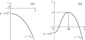
[latex]\sigma_k = \Re e(\lambda_{\vec k}) = \mu - \alpha (\Omega - k^2)^2,[/latex]

where [latex]k = \sqrt{k_x^2 + k_y^2} = ||\vec k||[/latex]. So each Fourier mode grows (or decays) at a rate that only depends on the magnitude [latex]k[/latex] of the associated wave vector [latex]\vec k[/latex], and not on its direction. If [latex]\mu < 0[/latex], all Fourier modes decay, and the solution [latex]\psi = 0[/latex] is linearly stable. As [latex]\mu[/latex] increases, some Fourier modes will become unstable.

If [latex]\Omega < 0[/latex], the graph of [latex]\sigma_k[/latex] as a function of [latex]k \ge 0[/latex] is monotonic (see Figure 10.3.a), and the first Fourier mode to become unstable is the [latex]k = 0[/latex] mode. This instability occurs for [latex]\mu = \alpha\, \Omega^2[/latex]. If on the contrary [latex]\Omega > 0[/latex], then [latex]\sigma_k[/latex] has a maximum for [latex]k = \sqrt \Omega \equiv k_c[/latex] (see Figure 10.3.b), and modes with [latex]k = k_c[/latex] become unstable when [latex]\mu[/latex] increases past zero. In this case, we expect a pattern to form above threshold with a characteristic length equal to [latex]l_c = 2 \pi / k_c[/latex]. The size of the system in which the pattern is to be observed should thus be much larger than [latex]l_c[/latex].

Above threshold, it is the nonlinear terms which decide which pattern is selected. Typically, if quadratic terms are present (i.e. if [latex]\zeta \ne 0[/latex] in Equation (10.1)), then hexagons are observed near threshold. On the contrary, if cubic terms dominate, then rolls (or stripes) prevail. If the imaginary parts of the coefficients in (10.1) are set to zero, the patterns that develop above threshold are stationary. If not, they are time-dependent. These and other aspects of the dynamics of Equation (10.1), including secondary instabilities and space-time disorder, may be explored with the MATLAB GUI interface called Patterns. This GUI allows the user to select the parameters and start a simulation from small, random initial conditions. Color-coded snapshots of the real part of the solution [latex]\psi[/latex] are shown at successive times as the simulation progresses. After a simulation has ended, new parameters can be entered and a new simulation may then be restarted from the last solution.

The theory of pattern formation^[10] provides means of describing the nonlinear dynamics of a pattern-forming system near and above threshold. A full discussion of this topic is however beyond the scope of these notes. In the next section, we briefly mention a reaction-diffusion model for the description of vegetation patterns in semiarid regions.

Vegetation patterns

In semiarid regions, plants (shrubs, grass, etc) tend to arrange themselves into stripes parallel to elevation contours on hilly terrain, and into patches on flat ground. Reaction-diffusion models have been proposed to explain these observations^[11][12][13]. In one of these articles, C.A. Klausmeier introduces a simple model with two dependent variables, the plant biomass [latex]n[/latex] and the amount of water [latex]w[/latex]. Written in dimensionless form, the model reads

[latex]\begin{align} \displaystyle \frac{\partial w}{\partial t} & = a - w - w\,n^2 + v \frac{\partial w}{\partial x}, \\ \displaystyle \frac{\partial n}{\partial t} & = w\,n^2 - m\, n + \left(\frac{\partial^2}{\partial x^2} + \frac{\partial^2}{\partial y^2}\right)n,\end{align}[/latex]

where [latex]a[/latex] represents water input through rain, [latex]v[/latex] is the speed at which water is transported downhill (in the [latex]-x[/latex] direction), [latex]w\, n^2[/latex] represents biomass increase due to water consumption, and [latex]m[/latex] is the plant death rate. Moreover, water evaporates at rate [latex]w[/latex], and the diffusion of [latex]n[/latex] accounts for the spreading of vegetation patches.

After finding equilibrium points (stationary and uniform solutions) of this model, the author investigates their linear stability. Figure 2 of the 1999 Klausmeier article shows a level set of the wavelength of the pattern that is expected to grow above threshold, in the [latex](a,m)[/latex] parameter plane, for a fixed value of [latex]v[/latex]. More precisely, the [latex](a,m)[/latex] plane can be divided into three regions, one where the fixed point corresponding to no vegetation is stable, one where the fixed point corresponding to homogeneous vegetation is stable, and a region in between where linear stability analysis predicts the existence of vegetation patterns. A numerical simulation of the model in this latter regime confirms the existence of traveling stripes on hilly terrain, and of vegetation patches on flat ground. The speed [latex]v[/latex] at which water flows downhill measures the steepness of the slope.

Summary

Different types of patterns may be obtained from the same, generic model, by choosing different sets of parameters. We have seen how to use linear stability analysis to predict whether a pattern can develop from a homogeneous solution as a control parameter ([latex]\mu[/latex] in the discussion of the Swift-Hohenberg equation) is varied, and if so, how to determine the typical length scale of the structure that will emerge. Although such a treatment is linear, it is nevertheless indicative of the kind of pattern one may expect. The same methodology, which consists in finding homogeneous solutions and studying their linear stability, can be applied to any pattern-forming system, as briefly illustrated in the case of the Klausmeier model.