The population of Red-tailed Hawks in the US

We start by analyzing data collected by the Audubon Society through its Christmas Bird Count. Counts are currently available for every year since 1900. This information is discrete (we are given the number of birds that were counted at the end of each year), imprecise (since not all of the birds were counted and different people participate in the counting effort every year), and necessarily reflects a combination of many factors (in particular, not just growth or decay due to births and deaths). We will focus on the data for the red-tailed hawk, which is a short-distance migrant.

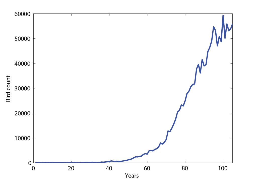
Figure 5.1 shows the number of red-tailed hawks that were counted in the US, from 1900 (year 1) to 2004 (year 105). We can see that the population grew during most of last century, and seems to have begun to saturate in the late nineties. In order to understand this data, we may try to plot the rate of change of the population, defined as

[latex]\displaystyle \frac{\Delta N}{\Delta t} = \frac{N(t + \Delta t) - N(t)}{\Delta t},[/latex]

where [latex]t[/latex] is time in years, [latex]N(t)[/latex] is the bird count at time [latex]t[/latex], and [latex]\Delta t = 1[/latex] year in this case. Such a graph shows that the quantity [latex]\Delta N / \Delta t[/latex] fluctuates and the size of its fluctuations increases with time. Since the number of red-tailed hawks also increases as a function of time, we can look instead at the rate of change normalized by the number of individuals, which we denote by [latex]R(t)[/latex]. We thus define the per capita rate of change of the red-tailed hawk population as

[latex]R(t) = \displaystyle \frac{N(t + \Delta t) - N(t)}{N(t) \Delta t}.[/latex]

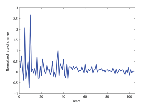
Figure 5.2 shows [latex]R(t)[/latex] as a function of [latex]t[/latex]. Fluctuations are of course still present, but they are now especially large only when [latex]N(t)[/latex] is relatively small. Moreover, the data appear to fluctuate about a mean value which is positive (although rather small). In the recent years, this trend breaks down, and from 1995 on, [latex]R(t)[/latex] seems to oscillate about a value closer to zero.

It is therefore reasonable to expect [latex]N(t+\Delta t)[/latex] to behave like a linear function of [latex]N(t)[/latex], up to some fluctuations, and to display saturation in the recent years. This is supported by the plot of Figure 5.3, which shows that [latex]N(t + \Delta t) = N(t+ 1)[/latex] as a function of [latex]N(t)[/latex]. We see that [latex]N(t+ 1)[/latex] is very close to [latex]1.025\ N(t)[/latex]. This slope was obtained by a least-square fit of the data with a straight line going through the origin (shown in red). As can be seen on Figure 5.3, the agreement is reasonably good. The value [latex]1.025[/latex] is also quite close to the 95% confidence interval [1.026, 1.029] for the per-annum growth rate of red-tailed hawks in North America, found in a 2016 article by C.S. Soykan et al.^[1], which uses statistical analysis to estimate population trends from bird counts.

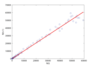
Note however that we do not expect – and in fact there is not – a good agreement at small values of [latex]N[/latex]. However, the scale of Figure 5.3 is such that the scatter of the points near the origin is not apparent for [latex]N(t) \lt 5,000[/latex], which corresponds to times [latex]t \le 50[/latex] (see Figure 5.1). In summary, even though the data is noisy and imprecise, a simple model for the red-tailed hawk population in the US from say 1950 to 1995 appears to be of the form

[latex]N (t + 1) = \kappa \ N(t),[/latex]

where [latex]\kappa[/latex] is a constant close to [latex]1.025[/latex]. We can understand such a linear relationship as follows. If we neglect migration in and out of the United States – recall that the red-tailed hawk is a short distance migrant, we can write

[latex]N(t + \Delta t) = N(t) + \text{number of births} - \text{number of deaths}.[/latex]

As a first approximation, it is reasonable to assume that both the number of deaths and the number of births may be written as the products of [latex]N[/latex] with a function of [latex]N[/latex] and [latex]t[/latex]. Such an approximation is valid for most population dynamics models in a closed system. We thus define the per capita birth rate  [latex]b,[/latex] and the per capita death rate  [latex]d[/latex] as

[latex]b = \displaystyle \frac{\text{number of births per }\Delta t}{N(t) \Delta t}, \qquad d = \displaystyle \frac{\text{number of deaths per }\Delta t}{N(t) \Delta t}.[/latex]

Then,

[latex]N(t + \Delta t) = N(t) \left(1 + b \Delta t - d \Delta t\right) = \kappa\ N(t),[/latex]

[latex]R(t)= \displaystyle \frac{N(t + \Delta t) - N(t)}{N(t) \Delta t} = b - d.[/latex]

In a developmental phase, that is when the number of individuals is much lower than the maximum population that can be sustained by the environment, one can assume that [latex]b[/latex] and [latex]d[/latex] are constant, which gives

[latex]N(t+1) = \kappa\ N(t), \qquad \kappa = \text{constant}.\qquad (5.1)[/latex]

For the red-tailed hawk, the above discussion suggests that [latex]\kappa \simeq 1.025[/latex], i.e. [latex]b - d = 0.025[/latex] individuals per year. Of course, fluctuations are always present in practice, but this simple model, known as the Malthus equation in discrete time, is sufficient to explain the exponential (or Malthusian) growth of the population. Indeed, Equation (5.1) implies that

[latex]N(t_0 + m \Delta t) = \kappa^m N(t_0).[/latex]

If [latex]\kappa > 1[/latex], i.e. if births exceed deaths, [latex]N(t)[/latex] grows exponentially. Conversely, if [latex]0 \lt \kappa \lt 1[/latex], [latex]N(t)[/latex] decays exponentially and the species is driven towards extinction. We have assumed that [latex]\kappa \ge 0[/latex]. If not, [latex]N(t)[/latex] would alternate between positive and negative values, and our population dynamics model would obviously be flawed.

When the number of individuals nears the carrying capacity of the environment, nonlinear effects can no longer be neglected, and the growth rate of the population changes with the number of individuals [latex]N(t)[/latex]. For instance, logistic growth corresponds to

[latex]\displaystyle N(t + \Delta t) = \Big(1 + \kappa \big(N_\infty - N(t)\big)\Big) \cdot N(t) \qquad \kappa = \text{constant},[/latex]

which has a [latex]N[/latex]-dependent per-[latex]\Delta t[/latex] growth rate equal to [latex]\Big(1 + \kappa \big(N_\infty - N(t)\big)\Big)[/latex]. The parameter [latex]N_\infty[/latex] represents the carrying capacity of the environment.

First-order difference equations

The example discussed above suggests that discrete population models are of the form [latex]N(t+\Delta t) = f(N(t))[/latex], or equivalently,

[latex]N_{k+1} = f(N_k), \qquad k \in \mathbb{N}, \qquad (5.2)[/latex]

where [latex]N_k= N(k \Delta t)[/latex]. Equation (5.2) is called a first order difference equation. It is linear if [latex]f(x)[/latex] is linear in [latex]x[/latex], and has constant coefficients if [latex]f[/latex] does not depend on [latex]k[/latex]. In the context of population dynamics, a model like Equation (5.2) is sometimes called a metered model. Equation (5.1), which can be written as

[latex]N_{k+1} = \kappa\ N_k,[/latex]

is therefore a linear first order difference equation with constant coefficients. As mentioned above, its solution is

[latex]N_k = \kappa^k\ N_0,[/latex]

where [latex]N_0[/latex] is the initial condition.

More generally, one can write

[latex]N_{k} = f^k(N_0),[/latex]

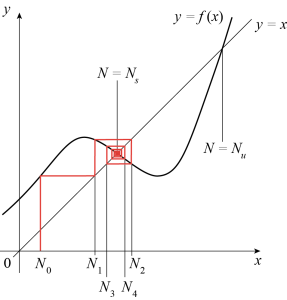
where [latex]f^k[/latex] is the [latex]k^{\text{th}}[/latex] iterate of [latex]f[/latex]. Even if the graph of [latex]f[/latex] is complicated, it is possible to visualize the dynamics of [latex]N_k[/latex] by iterating [latex]f[/latex] graphically, as shown in Figure 5.4. Starting from the initial value [latex]N_0[/latex] of [latex]N[/latex], we first find [latex]f(N_0)[/latex] as the [latex]y[/latex]-coordinate of the intersection of the graph of [latex]f[/latex] with the line [latex]x = N_0[/latex]. We then mark the value of [latex]N_1 = f(N_0)[/latex] on the [latex]x[/latex]-axis by drawing a vertical line through the intersection of the line [latex]x=y[/latex] with the line [latex]y = f(N_0)[/latex]. Finally, we repeat this process to find the successive iterates of [latex]f[/latex]. In the example of Figure 5.4, iterates starting at [latex]N = N_0[/latex] converge towards a fixed point [latex]N = N_s[/latex].

Fixed points and their linear stability

Fixed points [latex]N_c[/latex] of the map (5.2) are such that [latex]N_c = f(N_c),[/latex] and are found by intersecting the line of equation [latex]y = x[/latex] with the curve [latex]y = f(x)[/latex]. In the example of Figure 5.4, the function [latex]f[/latex] has two fixed points, [latex]N = N_s[/latex] and [latex]N = N_u[/latex]. We can study their linear stability as follows. Let [latex]N = N_c + u,[/latex] where [latex]u[/latex] is a small perturbation. Then,

[latex]f(N) = f(N_c + u) = f(N_c) + u f^\prime(N_c) + O(u^2),[/latex]

and

[latex]f(N) - N_c = f(N)-f(N_c) = u f^\prime(N_c) + O(u^2) \simeq u f^\prime(N_c),[/latex]

the last approximation being appropriate if [latex]u[/latex] is small enough. The linear map [latex]u_{k+1} = f^\prime(N_c) u_k[/latex] is such that its iterates converge towards zero if [latex]|f^\prime(N_c)| \lt 1[/latex], and diverge if [latex]|f^\prime(N_c)| \gt 1[/latex]. The fixed point [latex]N = N_c[/latex] is thus said to be linearly stable if [latex]|f^\prime(N_c)| \lt 1[/latex], and unstable if [latex]|f^\prime(N_c)| > 1[/latex]. If [latex]|f^\prime(N_c)| = 1,[/latex] [latex]N = N_c[/latex] is marginally stable.

The logistic map

As an example, consider the logistic map defined by Equation (5.2), with [latex]f(x) = a \ x \ (1 - x),[/latex] where [latex]a[/latex] is a parameter such that [latex]0 \lt a \lt 4[/latex]. If [latex]a \le 1[/latex], then [latex]x = 0[/latex] is the only non-negative fixed point. It is stable for [latex]a \lt 1[/latex] and marginally stable if [latex]a = 1[/latex]. For [latex]a > 1[/latex], there are two fixed points, [latex]x = 0[/latex] and [latex]x = 1 - 1/a[/latex]. Linear stability analysis shows that [latex]x = 0[/latex] is now unstable since [latex]a > 1[/latex], and that [latex]x = 1 - 1/a[/latex] is linearly stable if [latex]a \lt 3[/latex] and unstable if [latex]a > 3[/latex] (see exercises). A numerical exploration of the dynamics of the difference equation [latex]x_{n+1} = a\ x_n\ (1 - x_n)[/latex] reveals the presence of attractors of increasing complexity as [latex]a[/latex] is increased, such as period-two cycles (for instance at [latex]a = 3.2[/latex]), period-four cycles (e.g. at [latex]a = 3.5[/latex]), and period-eight cycles (for instance at [latex]a = 3.55[/latex]). In fact, a period-doubling cascade occurs as [latex]a[/latex] is increased, and the dynamics becomes chaotic near [latex]a = 3.57[/latex].

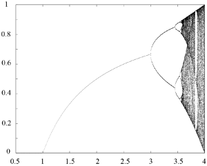
Figure 5.5 shows the bifurcation diagram of the logistic map. As mentioned above, for a given value of [latex]a[/latex], successive iterations of [latex]f[/latex] converge towards an attractor, for instance a fixed point, a period-two cycle, or a much more complicated structure. The bifurcation diagram of [latex]f[/latex] gives a representation of this attractor as a function of [latex]a.[/latex] It is numerically obtained by plotting the set of points

[latex]\left\{ x_k,\ k_{min} \lt k \lt k_{max} \right\},[/latex]

for different values of [latex]a[/latex]. Here, the initial condition is a point [latex]x_0 \in (0,1)[/latex], say [latex]x_0 = 1/2[/latex], [latex]k_{min}[/latex] is large enough so that the dynamics is sufficiently close to its attractor after [latex]k_{min}[/latex] iterations, and [latex]k_{max}[/latex] depends on the available computing power. The bifurcation diagram shown in Figure 5.5 was calculated with [latex]k_{min}=1500[/latex] and [latex]k_{max}=1700[/latex].

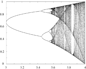
An enlargement for [latex]3 \le a \le 4[/latex] is shown in Figure 5.6. The cycles of period 2, 4 and 8 are clearly visible. Period 3 and 6 windows for larger values of [latex]a[/latex] are also easily detected.

A period-[latex]n[/latex] cycle may be analyzed by looking at fixed points of [latex]f^n[/latex]. Of course, as [latex]n[/latex] increases it quickly becomes difficult to solve for such fixed points. However, it can be shown that all of the period-doubling bifurcations occur in a similar, universal, fashion (see articles by P. Coullet & C. Tresser, 1978^[2] and by M. Feigenbaum, 1980^[3]). For a simple description of the various types of instabilities occurring in the logistic and other iterated maps, the reader is referred to the 1976 article by Robert May entitled Simple mathematical models with very complicated dynamics and to the exercises at the end of this chapter.

Continuous approximation of a one-species discrete model

The discrete model discussed in the first section is such that

[latex]\displaystyle \frac{N(t + \Delta t) - N(t)}{\Delta t} = N(t) R(t).[/latex]

As [latex]\Delta t \rightarrow 0[/latex], the difference quotient on the left-hand-side can be approximated by [latex]dN / dt[/latex], and we thus obtain the following continuous approximation

[latex]\displaystyle \frac{d N}{d t} = R(t) N(t). \qquad (5.3)[/latex]

Such an approximation is meaningful only if one can think of [latex]N[/latex] as a differentiable function of [latex]t[/latex]. In particular, [latex]N[/latex] must be continuous. Equation (5.3) will thus be a reasonable model for a population only if [latex]N[/latex] is large. In the case of a phenomenological model, if stochastic effects are negligible and [latex]N[/latex] approximates an actual number of individuals, the latter should be close to the integer [latex]\text{round}(N(t))[/latex] nearest to [latex]N(t).[/latex] Another possibility is to define [latex]N(t)[/latex] as a density, i.e. an average number of individuals per surface area for instance. Alternatively, one may view [latex]N(t)[/latex] as the expected value of a large population. In that context, it is useful to think of [latex]R(t) \delta t + O(\delta t^2)[/latex] as a per-capita probability of growth, so that the expected change in [latex]N[/latex] during the small amount of time between [latex]t[/latex] and [latex]t + \delta t[/latex] is [latex]R(t) N(t) \delta t + O(\delta t^2)[/latex]. In the rest of these notes, we mainly use continuous models and thus implicitly assume that the relevant quantities are adequately described by continuous variables.

Linear model

If [latex]R(t) = b - d \equiv r[/latex] with [latex]b[/latex] and [latex]d[/latex] constant, Equation (5.3) reads

[latex]\displaystyle \frac{d N}{d t} = r\ N(t) \qquad (5.4)[/latex]

and its solution is [latex]N(t) = \exp(r t) N_0,[/latex] where [latex]N_0[/latex] is the population at [latex]t = 0[/latex]. If [latex]r > 0,[/latex] the population grows exponentially; if [latex]r \lt 0,[/latex] [latex]N(t)[/latex] decays to zero and the species goes extinct. There is thus a direct analogy between the two linear models given by Equations (5.1) and (5.4), which is further explored in the exercises. Equation (5.4) is known as the Malthus equation in continuous time.

The Logistic model

Consider now the logistic model, given by

[latex]\displaystyle \frac{d N}{d t} = a N (N_c - N),[/latex]

where [latex]N_c[/latex] and [latex]a[/latex] are parameters. This equation, known as the Verhulst equation, can be simplified into

[latex]\displaystyle \frac{d M}{d t} =\lambda M (1 - M)\quad (5.5)[/latex]

by making the change of variables [latex]\displaystyle M = \frac{N}{N_c}[/latex] and [latex]\lambda = a N_c[/latex]. Note that [latex]M[/latex] is dimensionless and [latex][\lambda] = 1/T.[/latex] We could thus rescale the time variable and obtain a parameter-free model, but we will not do this now. The solution of Equation (5.5) with initial condition [latex]M(0) = M_0[/latex] is [latex]M(t) = \displaystyle \left[1 + \frac{1-M_0}{M_0} \exp(- \lambda t)\right]^{-1},[/latex] for all values of the parameter [latex]\lambda[/latex]. As [latex]t \rightarrow \infty[/latex], [latex]M \rightarrow 1[/latex] if [latex]\lambda > 0[/latex], for all values of [latex]M_0[/latex]. In terms of the original variables, we have [latex]N \rightarrow N_c[/latex]. The quantity [latex]N_c[/latex] is called the carrying capacity of the environment. It corresponds to an equilibrium state in which the number of deaths balances the number of births in order to sustain a population in the presence of limited resources. If [latex]\lambda \lt 0[/latex], then [latex]M \rightarrow 0[/latex] if [latex]M_0 \lt 1[/latex], and [latex]M \rightarrow \infty[/latex] for [latex]t \rightarrow t^*[/latex], where [latex]t^* = \displaystyle \frac{1}{- \lambda} \ln\left(\frac{M_0}{M_0-1}\right),[/latex] if [latex]M_0 > 1[/latex]. In this case, the solution therefore diverges in finite time. The dynamics of [latex]M[/latex] is monotonic for all values of [latex]\lambda[/latex], and is therefore completely different from that of the discrete logistic map, for which chaos may be observed.

General autonomous model

More generally, consider the differential equation

[latex]\displaystyle \frac{d N}{d t} = f(N), \qquad (5.6)[/latex]

where [latex]f[/latex] is a nonlinear function of [latex]N[/latex]. In the context of population dynamics, [latex]f(N)[/latex] is called the net growth rate of the population. It is often written as [latex]f(N) = N R(N)[/latex], where [latex]R(N)[/latex] is the net per capita growth rate of the population. Since the right-hand-side of Equation (5.6) does not depend on [latex]t[/latex], this differential equation is said to be autonomous.

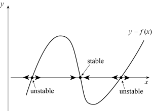
The fixed points [latex]N_c[/latex] of (5.6) are given by [latex]f(N_c)=0[/latex], and can be obtained graphically by looking at where the graph of [latex]f[/latex] intersects the horizontal axis. The nonlinear stability of these fixed points can also be assessed graphically. Indeed, [latex]f(N)[/latex] changes sign at [latex]N = N_c[/latex]. We know that if [latex]f(N) > 0[/latex] for [latex]N \lt N_c[/latex], then [latex]N[/latex] will grow towards [latex]N_c[/latex], whereas if [latex]f(N) > 0[/latex] for [latex]N > N_c[/latex], then [latex]N[/latex] will move away from [latex]N_c[/latex]. The stability of any fixed point [latex]N_c[/latex] of [latex]f[/latex] can thus be inferred by adding arrows to the horizontal axis that point to the left where [latex]f[/latex] is negative and to the right where [latex]f[/latex] is positive. A stable fixed point [latex]N_c[/latex] will have arrows pointing towards it on both sides, whereas an unstable fixed point will be associated with arrows pointing away from it. This is illustrated in Figure 5.7.

Discrete models with age distribution

Models with age distribution describe the number of individuals in each age group of a population and allow to take into account different birth and death rates for different subgroups. Consider for instance a three-group model, in which [latex]N_1(t)[/latex] is the number of children at time [latex]t[/latex]; [latex]N_2(t)[/latex] is the number of adults of child-bearing age, and [latex]N_3(t)[/latex] is the number of older adults. A simple set of difference equations describing the dynamics of such a population is as follows,

[latex]N_1(t + \Delta t) = N_1(t) + b_2 N_2(t) \Delta t - d_1 N_1(t) \Delta t - g_1 N_1(t) \Delta t[/latex]

[latex]N_2(t + \Delta t) = N_2(t) + g_1 N_1(t) \Delta t - d_2 N_2(t) \Delta t - g_2 N_2(t) \Delta t[/latex]

[latex]N_3(t + \Delta t) = N_3(t) + g_2 N_2(t) \Delta t - d_3 N_3(t) \Delta t,[/latex]

where [latex]d_i[/latex] is the per capita death rate of group [latex]i[/latex], [latex]g_i[/latex] is the rate at which surviving individuals move out of group [latex]i[/latex] (alternatively, [latex]g_i \Delta t[/latex] represents the probability that an individual in group [latex]i[/latex] will move to group [latex]i+1[/latex] during [latex]\Delta t[/latex]), and [latex]b_2[/latex] is the per capita rate at which individuals in group 2 give birth. The period of time [latex]\Delta t[/latex] could be one year or five years for human populations. It should be shorter than the typical timescales of the system being modeled, such as the time it takes for one child to become an adult, or the time it takes for a young adult to move to group 3.

The above system is linear and can thus be conveniently rewritten as a difference equation for the vector [latex]\vec C = (N_1,N_2,N_3)^T[/latex], which reads

[latex]\left(\begin{array}{c}N_1 \\ N_2 \\ N_3\end{array}\right)(t + \Delta t) = A \left(\begin{array}{c}N_1 \\ N_2 \\ N_3\end{array}\right)(t), \qquad (5.7)[/latex]

with [latex]A = \displaystyle \left(\begin{array}{ccc} 1 - (d_1 + g_1) \Delta t & b_2 \Delta t & 0 \\ g_1 \Delta t & 1 - (d_2 + g_2) \Delta t & 0 \\ 0 & g_2 \Delta t & 1 - d_3 \Delta t\end{array}\right).[/latex] The matrix [latex]A[/latex] typically has constant, non-negative entries. It is called a Leslie matrix in the context of population dynamics models. We can look for a solution to Equation (5.7) in the form [latex]\vec C (t_0 + m \Delta t) = r^m \vec C(t_0),[/latex] where [latex]t_0[/latex] is some initial time. Substitution of this expression into Equation (5.7) implies that [latex]\displaystyle A \vec C(t_0) = r\, \vec C(t_0),[/latex] i.e. [latex]\vec C(t_0)[/latex] is an eigenvector of [latex]A[/latex] with eigenvalue [latex]r[/latex]. If the matrix [latex]A[/latex] is diagonalizable, the general solution of Equation (5.7) may thus be written as

[latex]\vec C(m\, \Delta t) = a_1 r_1^m \vec C_1 + a_2 r_2^m \vec C_2 + a_3 r_3^m \vec C_3,[/latex]

where the [latex]\vec C_i[/latex] are three linearly independent eigenvectors of [latex]A[/latex] with associated eigenvalues [latex]r_i[/latex], and the [latex]a_i[/latex] are coefficients imposed by the initial condition [latex]\vec C(0) = \vec C_0[/latex], where [latex]\vec C_0[/latex] is known. Note that since [latex]A[/latex] has real entries, its eigenvalues are either all real or consist of a real eigenvalue and a complex conjugate pair of eigenvalues. In this latter case, two of the [latex]\vec C_i[/latex], say [latex]\vec C_2[/latex] and [latex]\vec C_3[/latex], are also complex conjugates and a real initial condition leads to [latex]a_3 = a_2^*[/latex], where the star denotes complex conjugation. The dynamics of Equation (5.7) depends on the position of the eigenvalues of [latex]A[/latex] in the complex plane, relative to the unit circle. Indeed, if [latex]|r_i|>1[/latex], then exponential growth will be observed in the direction of [latex]\vec C_i[/latex], with fastest and therefore dominant growth along the eigendirection associated with the principal eigenvalue of [latex]A[/latex]. Conversely, if all of the eigenvalues of [latex]A[/latex] have modulus less than 1, then [latex]\vec C(m\, \Delta t)[/latex] will converge towards zero. More complex behaviors, including chaos, may be observed if nonlinear effects are taken into account.

The LPA Model

Depending on the type of species whose populations is being modeled, effects other than births and deaths may have to be considered. As an illustration, we now discuss a model developed by R.F. Costantino and colleagues^[4][5][6] for a population of flour beetles, for which adults are known to eat their offspring. The different stages in the development of a beetle are the larval, pupal and adult stages. If one chooses [latex]\Delta t[/latex] (about 2 weeks for flour beetles) such that it corresponds to the time it takes on average for a larva to pupate and for a pupa to become a reproductive adult, one has, counting time in units of [latex]\Delta t[/latex], and in the absence of cannibalism,

[latex]\displaystyle \left\{\begin{array}{l} L(t + 1) = b A(t),\\ P(t + 1) = L(t) - d_l L(t),\\A(t + 1) = A(t) - d_a A(t) + P(t), \end{array}\right.[/latex]

where the positive constants [latex]d_l[/latex] and [latex]d_a[/latex] are the probabilities of death for larvae and adults during the period [latex]\Delta t\ (= 1)[/latex], the parameter [latex]b > 0[/latex] is the average number of eggs per adult that have hatched during [latex]\Delta t[/latex], and one has neglected deaths in the pupal stage.

Cannibalism of eggs by adults and larvae is modeled through multiplicative terms of the form [latex]\exp(-c_{ea} A(t))[/latex] and [latex]\exp(-c_{el} L(t))[/latex] respectively, and cannibalism of pupae by adults is described by [latex]\exp(-c_{pa} A(t))[/latex] (see the articles by Costantino et al. and Cushing et al. mentioned above). Here, the constants [latex]c_{ea}[/latex], [latex]c_{el}[/latex] and [latex]c_{pa}[/latex] are all positive. The exponential terms represent the fraction of eggs or pupae which survive to the next stage in their development, and can be understood as follows. Beetles in a crawling stage (larvae and adults) move through the flour and may encounter individuals in a non-moving stage, such as eggs and pupae. When this happens, the moving larva or adult beetle will bite the egg or pupa, thereby killing it. We assume that larvae only kill eggs, since pupae are bigger than larvae. Suppose the probability that an adult encounters one egg during the period of time [latex]\Delta t[/latex] is given by [latex]p\, \Delta t[/latex], where [latex]p[/latex] is constant. Then, the probability for this egg not to have been eaten by this adult at the end of [latex]\Delta t[/latex] is [latex]1 - p \Delta t[/latex], and the probability for this (or any other) egg to become a larva is then [latex]\left(1 - p \Delta t\right)^{A(t)}[/latex], since there are [latex]A(t)[/latex] adults. Thus, if eggs were only eaten by adults, one would write

[latex]L(t + \Delta t)=b A(t) (1 - p \Delta t)^{A(t)}=b A(t) \exp\left(A(t) \ln(1 - p \Delta t)\right)=b A(t) \exp\left(- c_{ea} A(t)\right),[/latex]

where [latex]c_{ea} = - \ln(1 - p \Delta t)[/latex]. Following similar arguments, the fact that eggs are also eaten by larvae is taken into account by multiplying the right hand side of the above equation by [latex]\exp(- c_{el} L(t))[/latex]. Therefore, the deterministic LPA model (where LPA stands for Larva, Pupa, Adult), which includes cannibalism of pupae and eggs by adults and of eggs by larvae, reads

[latex]\displaystyle \left\{\begin{array}{l} L(t + 1)=b A(t) \exp(-c_{ea} A(t) - c_{el} L(t)),\\ P(t + 1) = L(t) - d_l L(t),\\A(t + 1) = A(t) - d_a A(t) + P(t) \exp(-c_{pa} A(t)). \end{array}\right.[/latex]

A review of the dynamical properties of the LPA model can be found in the 2004 article by Jim Cushing et al. entitled Nonlinear population dynamics: models, experiments and data. In particular, it can be shown that the trajectories of the LPA model which start in the non-negative octant remain non-negative. Moreover, when stochastic terms are added to the above equations, the predictions given by the resulting model, including behavior consistent with chaotic dynamics, are in particular good agreement with experiments.

Summary

This chapter discusses discrete and continuous models for the dynamics of a single species. We first introduced exponential growth in the context of the Audubon Society’s count of red-tailed hawks in the United States, and added nonlinear saturation to the corresponding model. We then discussed fixed points and periodic cycles of one-dimensional nonlinear maps and saw that simple nonlinear difference equations, such as the logistic map, could have very complex dynamics and exhibit chaos. We also described linear and nonlinear population models with age groups. An example of the latter is the LPA model, whose stochastic version gives an accurate representation of experimental observations. Finally, we introduced continuous models as approximations of discrete models, discussed the global stability of their fixed points, and pointed out that one-dimensional (as well as two-dimensional) continuous models have very simple dynamics. In particular, they cannot exhibit chaos.

The methods and techniques introduced in this chapter generalize to more complex situations. The exercises below discuss models with continuous age distributions, delay and harvesting, as well as the evolution of the population of the United States.