Predator-prey models: the Lotka-Volterra equations

Consider a closed system involving a population of predators (e.g. sharks) and prey (e.g. little fish). Let [latex]F[/latex] represent the density of prey and [latex]S[/latex] that of the predator. It is clear that if there is abundant prey, predators will proliferate. As a consequence, more prey will be eaten and [latex]F[/latex] will decrease, but so will [latex]S[/latex] since there will be less food for the predators. However, if [latex]S[/latex] decreases, [latex]F[/latex] will have a chance to grow again since the prey will not be eaten as much. This reasoning suggests that parameter values may exist for which [latex]F[/latex] and [latex]S[/latex] oscillate in time^[1][2].

If we neglect migration, and assume that [latex]F[/latex] and [latex]S[/latex] are the only dependent variables – in particular we assume that there is an ample (but not infinite) supply of nutrients for the prey, we may write

[latex]\displaystyle \left\{\begin{align} \displaystyle \frac{dF}{dt} &=F \left(\alpha - \beta F - \gamma S \right) \equiv g(F,S),\\ \displaystyle \frac{dS}{dt} &= S \left( - \kappa + \delta F \right) \equiv h(F,S), \end{align}\right. \qquad (6.1)[/latex]

where the constant parameters [latex]\alpha[/latex], [latex]\beta[/latex], [latex]\gamma[/latex], [latex]\kappa[/latex] and [latex]\delta[/latex] are all non-negative. This model indicates that when [latex]S = 0,[/latex] the prey population evolves according to a logistic model, and that when [latex]S \ne 0[/latex], prey are eaten proportionally to both their own abundance ([latex]F[/latex]) and that of the predators ([latex]S[/latex]). The predators have a growth (birth minus death) rate equal to [latex]-\kappa[/latex] if [latex]F=0[/latex]. Since [latex]\kappa[/latex] is positive, this means that in the absence of prey, the predator population would be driven to extinction. The growth rate of [latex]S[/latex] is then corrected by a linear term [latex]\delta\, F\, S[/latex], proportional to [latex]F[/latex].

If [latex]\beta = 0[/latex], this model is called the Lotka-Volterra system (see footnotes 1 and 2 for references) and is the simplest continuous model that incorporates the basic factors describing the interaction of a predator and its prey. It should be considered as a starting point for more complicated and more realistic models. The rest of this section is devoted to an analysis of Equations (6.1).

Scalings

Equations (6.1) involve three variables, [latex]F[/latex], [latex]S[/latex] and [latex]t[/latex], and five parameters, which we assume are positive (except possibly for [latex]\beta[/latex]). Scaling all of the variables should allow us to reduce this system to a problem with two (i.e. five minus three) parameters. A typical value for [latex]F[/latex] is given by [latex]F_0 = \kappa / \delta[/latex] (see the second equation of (6.1)), and a typical value for [latex]S[/latex] can be chosen as [latex]S_0 = \alpha / \gamma[/latex] in a similar fashion. For a characteristic time, we may take [latex]\tau = 1 / \kappa[/latex]. Then, if we define [latex]\displaystyle f = \frac{F}{F_0},[/latex] [latex]\displaystyle s = \frac{S}{S_0},[/latex] and [latex]\tau = \kappa t,[/latex] we obtain a dimensionless, canonical model, which reads

[latex]\displaystyle \left\{\begin{align} \displaystyle \frac{d f}{d \tau} & = a f (1 - b f - s),\\ \displaystyle \frac{d s}{d \tau} & = s (-1 + f), \end{align}\right. \qquad (6.2)[/latex]

Here, the parameters [latex]a[/latex] and [latex]b[/latex] are related to the original parameters by [latex]\displaystyle a = \frac{\alpha}{\kappa}[/latex], [latex]\displaystyle b = \frac{\beta \kappa}{\alpha \delta},[/latex] and are therefore positive.

Phase plane analysis

A description of the phase plane associated with system (6.2) gives us a qualitative understanding of the predator-prey equations. With this information, we are able to address questions such as those listed below, even if we do not have explicit forms for all of the solutions of (6.2).

• Is it possible for the populations of sharks or little fish to go extinct?
• Does the model make biological sense?
• Can oscillations be observed?

Before going any further, it is important to check that the model is “biologically well-posed,” i.e. that if [latex]s[/latex] and [latex]f[/latex] are initially non-negative, they will remain so. Assume for instance that [latex]s=0[/latex]. Then, the second equation of (6.2) indicates that [latex]s[/latex] will remain zero. Trajectories in the [latex](f,s)[/latex] plane are therefore along the [latex]f[/latex] axis or away from it, but do not cross this axis. Similarly, the first equation of (6.2) shows that trajectories do not cross the [latex]s[/latex] axis.

We now turn to a description of the phase portrait of system (6.2). The fixed points of this system are given below in terms of their coordinates in the [latex](f,s)[/latex] plane. They are

[latex]\displaystyle P_0 = (0, 0), \qquad P_1 = \left(\frac{1}{b}, 0\right), \qquad P_2 = (1, 1 - b),[/latex]

and are all located in the first quadrant provided [latex]0 \lt b \le 1[/latex], which we will assume is true. Linear stability analysis can be used to describe the local dynamics of (6.2) near its three fixed points. The Jacobian of (6.2) is given by

[latex]J(f,s) = \displaystyle \left(\begin{array}{cc} a (1 - 2 b f - s) & - a f \\ s & -1 + f \end{array} \right).[/latex]

Analysis near the origin, [latex]P_0[/latex]

For [latex]P_0[/latex], [latex]s = f = 0[/latex] and the Jacobian [latex]J(0,0)[/latex] is diagonal. Its eigenvalues are [latex]a[/latex] and [latex]-1[/latex], with associated eigenvectors [latex]\displaystyle \left(\begin{array}{c}1 \\ 0 \end{array}\right)[/latex] and [latex]\displaystyle \left(\begin{array}{c}0 \\ 1 \end{array}\right)[/latex] respectively. The origin is therefore a saddle point.

Analysis near [latex]P_1[/latex]

For [latex]P_1[/latex], [latex]f = 1/b[/latex] and [latex]s = 0.[/latex] The Jacobian [latex]J(1/b,0)[/latex] is an upper-triangular matrix and its eigenvalues are therefore its diagonal entries. They are [latex]-a[/latex] and [latex]-1+1/b[/latex]. Since [latex]b \le 1[/latex], this fixed point is also a saddle (with possibly a neutral direction if [latex]b = 1[/latex]). The eigenspace associated with [latex]-a[/latex] is spanned by [latex]\displaystyle \left(\begin{array}{c}1 \\ 0 \end{array}\right)[/latex], and the eigenspace associated with [latex]-1+1/b[/latex] is spanned by [latex]\displaystyle \left(\begin{array}{c}1 \\ (-a b + b- 1)/a \end{array}\right)[/latex].

Analysis near [latex]P_2[/latex]

For [latex]P_2[/latex],  [latex]f = 1[/latex] and [latex]s = 1 - b[/latex]. The Jacobian [latex]J(1,1 - b)[/latex] reads

[latex]\displaystyle J(1 - b, 1) = \left(\begin{array}{cc} -a b & -a \\ 1 - b & 0 \end{array} \right),[/latex]

and its eigenvalues [latex]\lambda_1[/latex] and [latex]\lambda_2[/latex] are such that

[latex]\det(J) = \lambda_1 \lambda_2 = \det\left[J(1-b,1)\right] = a (1 - b) > 0,[/latex]

and

[latex]\hbox{Tr}(J) = \lambda_1 + \lambda_2 = \hbox{Tr}\left[J(1-b,1)\right] = - a b \lt 0.[/latex]

Therefore [latex]P_2[/latex] is either a stable node or a stable spiral.

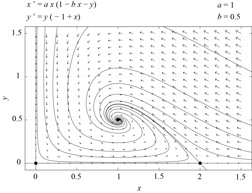
This analysis thus indicates that if the initial values of [latex]f[/latex] and [latex]s[/latex] are positive, then the dynamics will converge to the fixed point [latex]P_2[/latex], for which both shark and fish populations are of finite size. In other words, no periodic oscillations are observed. Figure 6.1 shows the phase plane of system (6.2) for [latex]a=1[/latex] and [latex]b=0.5[/latex], obtained with PPLANE. In this case, the fixed point [latex]P_2[/latex] is a stable spiral.

As an exercise, the reader should work out the case where [latex]b > 1[/latex], for which only two of the fixed points are in the first quadrant. Then, [latex]P_1[/latex] is a stable node and all initial conditions with [latex]f > 0[/latex] and [latex]s > 0[/latex] converge to [latex]P_1[/latex]. In this situation, the sharks are extinct and the fish have reached the carrying capacity of the environment they live in.

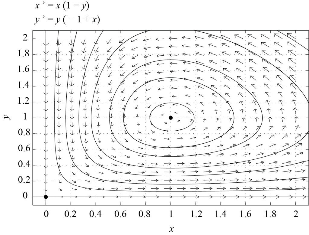
It is possible to observe oscillations, provided we set [latex]b = 0[/latex]. This is indeed a necessary condition if we want [latex]P_2[/latex] to be a center, since Tr[latex](J(P_2)) = - a b[/latex] and [latex]\det(J(P_2)) = a (1 - b)[/latex]. Indeed, setting [latex]b =0[/latex] makes the trace of [latex]J(P_2)[/latex] vanish, but keeps its determinant positive. In this case, [latex]P_1[/latex] disappears (it is in fact sent to infinity as [latex]b[/latex] goes to zero), and we are left with two fixed points, [latex]P_0 = (0, 0)[/latex] and [latex]P_2 = (1, 1)[/latex]. The Jacobian [latex]J(1,1) = \left(\begin{array}{cc} 0 & -a \\ 1 & 0 \end{array} \right)[/latex] has eigenvalues [latex]\pm i \sqrt a[/latex], so [latex]P_2[/latex] is now a linear center, as expected. Figure  6.2 shows the corresponding phase plane, with closed trajectories around [latex]P_2[/latex]. We can prove the existence of close trajectories as follows. Any trajectory in the phase plane is such that

[latex]\displaystyle \frac{d f}{d s} = \frac{a f (1 - b f - s)}{s (-1 + f)}.[/latex]

When [latex]b = 0[/latex], an implicit solution to this equation is

[latex]\displaystyle \left(f \exp(-f) \right) \left(s \exp(-s)\right)^a = \zeta,[/latex]

where [latex]\zeta[/latex] is a non-negative constant. It is easy to see that there are values of [latex]\zeta[/latex] for which this equation defines a closed curve around [latex]P_2[/latex]. Indeed, the function [latex]x \exp(-x)[/latex] is zero at the origin, has a maximum equal to [latex]1/e[/latex] at [latex]x=1[/latex], and goes to zero as [latex]x \rightarrow \infty[/latex]. As a consequence, for given values of [latex]s[/latex] and [latex]a[/latex], one can find a range of values of [latex]\zeta[/latex] such that the equation [latex]f \exp(-f) = \displaystyle \frac{\zeta}{\left( s \exp(-s) \right)^a}[/latex] has two solutions, one on each side of [latex]f = 1[/latex]. A similar reasoning applies to cross-sections parallel to the [latex]s[/latex]-axis. These closed trajectories are drawn counterclockwise in the first quadrant of the [latex](f,s)[/latex] plane, since

[latex]\displaystyle \frac{d f}{d \tau} = a f (1 - s) > 0 \Leftrightarrow s \lt 1 \text{ and }\frac{d s}{d \tau} = s (-1 + f) > 0 \Leftrightarrow f > 1.[/latex]

The Lotka-Volterra model therefore predicts periodic oscillations of the predator and prey populations.

The ideas developed in this section can be generalized to more complex systems. For instance, it is shown in a 2000 article by G.F. Fussmann et al. entitled Crossing the Hopf Bifurcation in a Live Predator-Prey System, that the predictions of a predator-prey model involving environmental factors as well as reproductive and non-reproductive fractions of a population compare very well with experimental results.

Two competing species

We now turn to the problem of two species competing for the same resources. We will assume that in the absence of the other species, each species grows according to a logistic law. The competition for food makes the growth rate of each species limited by the presence of the other. As a first approximation, this effect is linear. If we denote by [latex]X[/latex] and [latex]Y[/latex] the average density of each species, we thus have

[latex]\displaystyle \left\{\begin{align} \displaystyle \frac{dX}{dt} & = X (\alpha - \beta X - \gamma Y), \\ \displaystyle \frac{dY}{dt} & = Y (\delta - \kappa Y - \zeta X), \end{align}\right. \qquad (6.3)[/latex]

where [latex]\alpha[/latex], [latex]\beta[/latex], [latex]\gamma[/latex], [latex]\delta[/latex], [latex]\kappa[/latex] and [latex]\zeta[/latex] are positive parameters. As for the Lotka-Volterra model, we first rescale these equations in order to reduce the number of independent parameters. We then perform a phase plane analysis to describe the dynamics of the competing species.

Scalings

Characteristic values of [latex]X[/latex] and [latex]Y[/latex] are [latex]X_0 = \alpha/\beta[/latex] and [latex]Y_0 = \delta / \kappa[/latex]. A characteristic time is for instance [latex]t_0 = 1/\alpha[/latex]. So we can define dimensionless quantities as

[latex]\displaystyle x = \frac{X}{X_0}, \qquad y = \frac{Y}{Y_0}, \qquad \tau = \frac{t}{t_0},[/latex]

substitute these expressions into Equations (6.3), and look for a simplified system for the variables [latex]x[/latex] and [latex]y[/latex]. We obtain

[latex]\displaystyle \left\{\begin{align} \displaystyle \frac{dx}{d \tau} & = x\, (1 - x - a\, y),\\ \displaystyle \frac{dy}{d \tau} & = c\, y\, (1 - y - b\, x), \end{align}\right. \qquad (6.4)[/latex]

where [latex]\displaystyle a = \frac{\gamma \delta}{\alpha \kappa},[/latex] [latex]\displaystyle b = \frac{\zeta \alpha}{\beta \delta},[/latex] and [latex]\displaystyle c = \frac{\delta}{\alpha}.[/latex] We thus have a three-parameter model. This was to be expected since we initially had a six-parameter nonlinear system, and had the possibility of rescaling three variables, [latex]t[/latex], [latex]X[/latex] and [latex]Y[/latex]. We leave the question of biological well-posedness as an exercise and directly move to an analysis of the fixed points of Equations (6.4).

Phase plane analysis

As usual, fixed points are obtained by solving [latex]x(1 - x - a y) = 0[/latex] and [latex]y (1 - y - b x) = 0.[/latex] This system of equations has four solutions, given by

[latex]P_0 = (0,0), \quad P_1 = (1, 0), \quad P_2 = (1, 0), \quad P_3 = \displaystyle \left(\frac{1 - a}{1 - a b},\frac{1 - b}{1 - a b}\right).[/latex]

The last fixed point [latex]P_3[/latex] is in the first quadrant only if [latex]1-a[/latex], [latex]1 - b[/latex] and [latex]1 - a b[/latex] are all of the same sign, and [latex]a b \ne 1[/latex]. In what follows, we assume that these conditions are satisfied, and denote by [latex]\epsilon = \pm 1[/latex], the sign of any of these three quantities, i.e.

[latex]\epsilon = \text{sign}(1 - a) = \text{sign}(1 - b) = \text{sign}(1 - a b).[/latex]

The Jacobian of (6.4) is

[latex]J(x,y) = \displaystyle \left(\begin{array}{cc} 1 - 2 x - a y & - a x \\ - b \, c \, y & c (1 - 2 y - b x)\end{array} \right).[/latex]

We can now calculate the eigenvalues of [latex]J(x,y)[/latex] evaluated at each of the fixed points.

Analysis near the origin, [latex]P_0[/latex]

For [latex]P_0,[/latex] [latex]J(0,0)[/latex] is diagonal and its eigenvalues are [latex]1[/latex] and [latex]c[/latex]. Since they are both positive, the origin is an unstable node.

Analysis near [latex]P_1[/latex]

For [latex]P_1,[/latex] [latex]J(1,0)[/latex] is upper-triangular, and its eigenvalues are [latex]-1[/latex] and [latex]c (1-b)[/latex]. If [latex]\epsilon = 1,[/latex] then [latex]P_1[/latex] is a saddle. If [latex]\epsilon = -1[/latex], it is a stable node.

Analysis near [latex]P_2[/latex]

For [latex]P_2,[/latex] [latex]J(0,1)[/latex] is lower-triangular, and its eigenvalues are [latex]1 - a[/latex] and [latex]-c[/latex]. Thus [latex]P_2[/latex] is a saddle if [latex]\epsilon = 1[/latex], and a stable node if [latex]\epsilon = -1[/latex].

Analysis near [latex]P_3[/latex]

For [latex]P_3[/latex], the Jacobian is

[latex]\displaystyle J \left( \frac{1 - a}{1 - a b}, \frac{1 - b}{1 - a b} \right) = \displaystyle \frac{1}{1 - a b} \left(\begin{array}{cc} a-1 & a\, (a-1) \\ b\,c\,(b-1) & c\,(b-1)\end{array} \right).[/latex]

Since its trace [latex]T[/latex] and determinant [latex]D[/latex] are given by

[latex]\displaystyle T = \frac{1}{1 - a b} \left(a - 1 + c (b -1)\right), \quad D = \frac{(a - 1) c (b - 1)}{1 - a b},[/latex]

we see that [latex]\text{sign}(T)=-1[/latex] and [latex]\text{sign}(D)=\epsilon.[/latex] If [latex]\epsilon = -1[/latex], [latex]P_3[/latex] is a saddle. If [latex]\epsilon = 1[/latex], [latex]P_3[/latex] is a stable node. Indeed, the discriminant of the characteristic polynomial is

[latex]T^2 - 4 D = \displaystyle \frac{1}{(1- a b)^2} \left[ (a-1) - c (b-1) \right]^2,[/latex]

and is therefore positive. Thus, both eigenvalues are real.

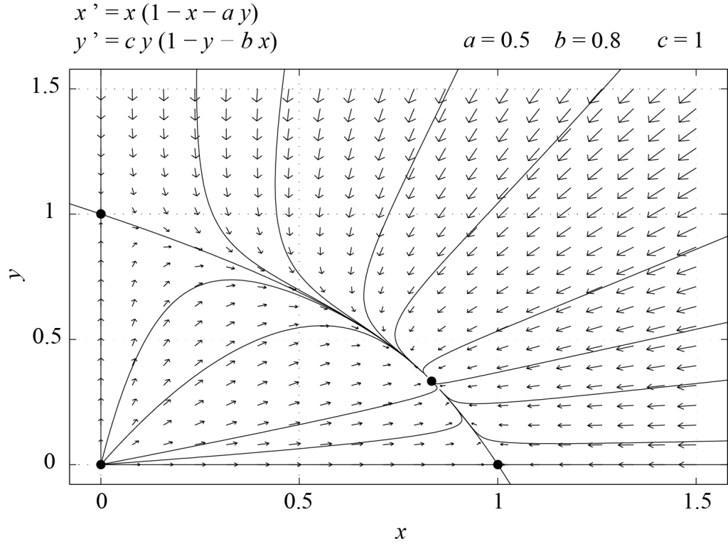
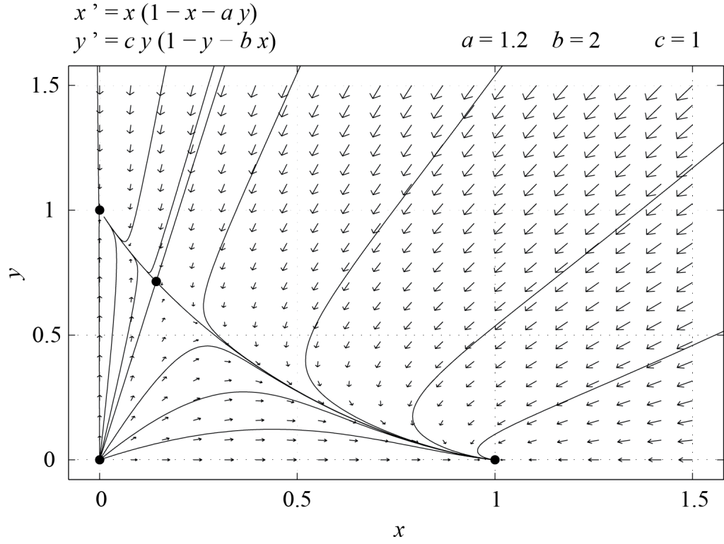
Figures 6.3 and 6.4 show phase portraits of system (6.4) for [latex]\epsilon = 1[/latex] and [latex]\epsilon = -1[/latex] respectively.

From an ecological point of view, the two species coexist if [latex]P_3[/latex] is stable, i.e. if [latex]\epsilon = 1[/latex]. If not, then one of the species is driven to extinction by the other, since the only fixed points which are stable when [latex]\epsilon = -1[/latex] are [latex]P_1[/latex] and [latex]P_2[/latex], for which one of the populations is zero. From this simple example, we see how relationships between model parameters may be inferred from biological facts. For instance, the above analysis indicates that if the two species coexist, then [latex]a \le 1[/latex] and [latex]b \le 1,[/latex] with [latex]a b \ne 1.[/latex]

Summary

In this chapter, we introduced two classical population dynamics models, the predator-prey system and a system describing two species competing for the same resources. The main tool we used for the analysis of these two-dimensional models was phase plane analysis. We only discussed elementary continuous models, but discrete analogues as well as more complex models may of course be considered.

From a biological point of view, it is important to remember that predator-prey systems may exhibit temporal oscillations. The latter typically arise from a Hopf bifurcation, as discussed for instance in the paper by Fussmann et al.^[3] (see exercises), and are not related to the presence of an infinite number of closed orbits, as was the case in the Lotka-Volterra system with [latex]a = 1[/latex] and [latex]b = 0[/latex].

In the case of competing species, the simple model presented in this section shows that the two species can only coexist if [latex]a[/latex] and [latex]b[/latex] in system (6.4) are both less than unity. Otherwise, one of the species will drive the other to extinction.