
21 Forces and Force Diagrams
Before continuing with forces, I want us to do a constant acceleration problem as a review. I don’t want us to forget how to handle those.
Exercise 21.1: A Toy Car
A toy car accelerates has a spring mechanism that allows it to move on its own. When you wind it up, the car accelerates at  for 4 seconds to the right. At that point, the energy in the spring is used up, and the car slowly slows down with an acceleration of
  until it stops. Find how far the car travels before coming to a stop.
Hint: This problem has not one, but TWO mini-stories. You should treat each mini-story as its own little problem.
There is an important lesson here: a problem can have more than one mini-story going on. If so, you need to make sure you treat each of the little mini-stories as their own problem. We’ll see much more of this as we progress in this class.
Let’s get back to forces. In the previous chapter, we learned that the motion of objets subject to a constant force is given by the kinematic equations. This is not particularly useful if there are no constant forces in the Universe. Fortunately, there are many every-day phenomena that can be approximated using constant forces. We’ll go through several examples, starting with perhaps the most famous one: gravity.
Exercise 21.2: Falling Objects
If you pick an object up and let it go, it falls down. But- does the object drop at constant speed? Let’s figure it out.
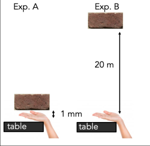 If I tell you I’m going to drop a brick on your hand, would you rather I drop the brick from a height of 1 mm (experiment A), or a height of 20 m (experiment B)?
Surely, we would all choose the 1 mm; it will hurt less. But why will it hurt less? What does this tell you about the brick’s velocity as it falls?
The point here is that objects pick up speed as they fall. That is, falling objects are accelerating. Therefore, there must be a force pushing down on the object. We call this force gravity. The force of gravity on a specific object is called the object’s weight.
You will remember from the previous chapter than whenever we solve problems involving forces, we must draw all the forces acting on an object. However, this is not quite the complete rule. The complete rule is as follows:
When drawing forces, you should always have the arrow either start or end at the point at which the force is being applied.
Let’s use gravity as an example.
Example: A Force Diagram for Gravity
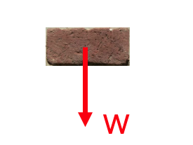
Gravity “pulls from the middle.” We will justify this statement later in class, but for now we’ll just take it for granted. Given this, to draw the force of gravity on a brick, I’d draw an arrow that starts at the middle of the brick, as shown at right.
Drawing forces at the location at which they are applied serves two purposes: 1) it helps better represent what’s actually happening in a problem; and 2) while the information of where a force is applied is not really important for our current discussion, this information will become critical when we start solving rotational problems.
Bottom line: always draw forces at the point at which they are applied.
To end, I want to highlight one critically important fact about forces, namely that
All forces are applied by “something”.
This is always true; E.g. I push you. There are no such things as disembodied forces: the sentence “push you” doesn’t mean anything When dealing with forces, you should always know who is pushing on what.
In the case of gravity, the thing doing the pushing is the Earth itself: the Earth pulls everything around it straight down. Moreover, that pulls is very nearly constant for every day objects. Thus, we can approximate gravity as a constant downwards force. We’ll have more to say about gravity in the next chapter.
Exercise 21.3: Review
One  more flashback to simple harmonic motion. Consider a pendulum bobbing back and forth. You are probably not surprised that this “bobbing” motion can be described as simple harmonic motion. Let’s see how:
Consider the angle  that the pendulum makes with the vertical line, so
  is the equilibrium position. We will make positive when the angle opens to the right, and negative when it opens to the left.
The pendulum shown above has a period of 2.8 s, and has a maximum opening angle  . Determine the amplitude and angular frequency of the oscillation, and write an expression for
  assuming the particle starts at maximum displacement at
  .
.
Key Takeaways