
18 Motion With Constant Acceleration
In the previous two chapters, we defined acceleration via the relation  , and tried to get some intuition for how acceleration worked. We now further build our intuition by discussing what motion with constant acceleration looks like.
Exercise 18.1: Motion Subject to a Constant Acceleration
Suppose an object starts at a position  and with a velocity
  at some initial time
  . The object moves with a constant acceleration
  .
.
1. What will the object’s velocity at an arbitrary time  later be?
2. Suppose the object started at position  . Now that you have calculated the velocity of the particle at an arbitrary time later, find the position
  at an arbitrary time later.
Let us summarize what we just found. We looked at the motion of an object with constant acceleration. By integrating the equation  (and
(and  ), we figured out both the position and velocity of the object as a function of time. These equations are called the kinematic equations. If we further assume that the initial time is zero (i.e.
  these equations become:


These are the kinematic equations. Notice that the only assumption that goes into these equations is “constant acceleration.” Therefore,
Every problem with constant acceleration can be solved using the kinematic equations.
Conversely,
If an object does NOT have constant acceleration, you should not use the kinetic equations.
Also note that the equations above are vector equations; that is, they are not really one equation, but one equation per component. For instance, along the  -axis we have


where  and
and  are the initial velocity and acceleration along the x-axis. If a particle is experiencing constant acceleration along the
  -axis, then a similar set of equations hold for the -axis.
Let’s solve a problem with constant acceleration to see how we can use the kinematic equations.
Exercise 18.2: Tesla Joy Ride
A Tesla roadster goes from 0 mph to 60 mph in 1.9 seconds (60 mph is about 26.8 m/s). This is quite a high acceleration, as should be clear from the following video:
Assuming the Tesla moves with constant acceleration, find the distance the vehicle has covered by the time it reaches 60 mph.
We’ll do this problem together. Before we start with step 1 of the three steps of problem solving, I want you to take the time to summarize the story of the problem. This story has a clear beginning and end, so make sure you identify these end points.
Step 1: Draw a picture. The picture should include all of the information in the problem! If you’re stuck, look at my solution, and fix anything that needs fixing so you can move on to step 2.
Step 2: Find relations. Given the conditions of the problem, what are the relations that hold between the variables included in your picture?
If you’re stuck, you can look at my solution, and fix anything that needs fixing before moving on.
Step 3: Solve unknowns. Use the equations you found above to solve for the variables you were not given. Try it, and then compare to my answer.
The problem above should help you see just how important it is to have a good understanding of the story behind the problem. This is so much so, that from now on, I will officially add a “step 0” to the rules of problem solving. The four steps of problem solving are:
- Step 0: What’s the story?
- Step 1: Draw a picture.
- Step 2: Find Relations.
- Step 3: Solve Unknowns.
I also want you to notice that when solving the problem, we ended up using the kinematic equations to relate the beginning of the problem to the end of the problem. I find that this is the most useful way of thinking about the kinematic equations. Consequently, from this point on I will write the kinematic equations as follows:
 .
.
 .
.
The subscript “f” stands for “final”, and  is the time between the start of the problem and the end of the problem. Here,
  and are the initial velocity and acceleration along the x-axis, respectively.
Throughout this book, you will occasionally run into tablets like the ones below.
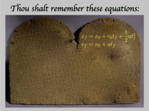
These tablets contain equations that you absolutely should know by the end of this class/book. I hope you will find that the number of equations you need to remember is, in fact, very small.
Exercise 18.3: Stopping a Bullet
Let’s start by looking at the following video (original video here).
A 50 caliber desert eagle shoots bullets at  . As you saw in the video, the bullets are stopped by
  of sand. Each bullet has a mass of
  .
.
How long does it take for the bullet to stop as it travels through the sand?
Try solving the problem, starting with step 0: What is the story?
Now step 1: Draw a picture.
Now bring it home: find relations and solve unknowns.
D. The barrel of a desert eagle 50 caliber gun is 6 in long. Which acceleration is larger in magnitude, the acceleration of the bullet as it shoots out of the gun, or the bullet’s acceleration as it is stopped by the sand? Explain you answer in English: you don’t need to do any algebra.
Key Takeaways
The motion of objects with constant acceleration is described by the kinematic equations. Write down these equations from memory.
Practice Problems
PP 18.1: A car is driving at 60 mph down the highway. At that speed, the typical stopping distance of a car is 55 m. How long does it take for a car to break this distance?
PP 18.2: The Falcon 9 rocket developed by Space X is a two stage rocket. During the first stage, the rocket accelerates upwards for a total time of  , at which point it jettisons its large boosters. At this point, the rocket is traveling at a speed of
  . What is the altitude of the Falcon 9 rocket at the end of Stage 1?