Velocity

8 Velocity

We have learned how to use vectors to describe the position and displacement of an object. We can now turn to describing how objects move. The movement of an object is described by its velocity. The velocity tells us:

how fast an object is moving.
in which direction is the object moving.

The fact that velocity is a vector is pretty important: traveling at 60 mph due East is not at all the same thing as traveling 60 mph due North! For this reason, in physics we make a distinction between the words velocity and speed.

Velocity is a vector (how fast you’re going, and in which direction).

Speed is a scalar (how fast you’re going, regardless of direction).

Thus, 60 mph due North is a velocity, but 60 mph is a speed.

Exercise 8.1: What is Constant Velocity?

Ok- so velocity is a vector, and we care both about its magnitude and direction. But what exactly is velocity in math terms? To figure it out, let’s think about an object moving in space. At any given time, there is a vector $\vec r(t)$ that starts at the origin and points to the object. We call this the position vector. As the object moves, it traces out a curve, so you get something that looks like this:

Consider the particle at time $t$ and position $\vec r(t)$ . Some small amount of time $\Delta t$ later, the particle’s position is $\vec r(t+\Delta t)$ . From our every day experience, we know

(distance travelled) = (speed) $\times$ (time).

Based on the above expression, what are the units of velocity?

We can use this intuition of (distance travelled) = (speed) $\times$ (time) to define the velocity vector. Let’s see how this comes about.

Exercise 8.2: The Definition of Velocity

Consider a particle moving along a trajectory $\vec r(t)$ as shown below, and let’s draw the position vectors $\vec r(t)$ and $\vec r(t+\Delta t)$ . We will also draw a vector $\vec s$ going from $\vec r(t)$ to $\vec r(t+\Delta t)$ . This vector $\vec s$ is telling us how the particle moved.

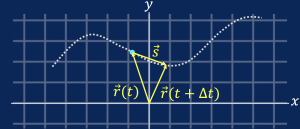
A. Find the relation between the vectors $\vec r(t)$ , $\vec r(t+\Delta t)$ , and $\vec s$ .

B. Use the idea that (distance travelled) = (velocity) $\times$ (time travelled) to relate the vector $\vec s$ and the velocity vector $\vec v$ of the particle.

C. Plug in your result from part B into the relation you found in part A to find how the velocity vector $\vec v$ is related to $\vec r(t)$ and $\vec r(t+\Delta t)$ .

The equation you just derived, i.e. $\vec r(t+\Delta t) = \vec r(t)+\vec v \Delta t$ , is the best way to think about velocity. In particular, notice that in English, this equation can be rewritten as:

(Final position of a particle) = (initial position) + (distance moved)

where (distance moved) = $\vec v\Delta t$ .

In the next two problems, we use this new understanding to learn an interesting feature about which way the velocity of an object points.

Exercise 8.3: Which Way Does Velocity Point?

Consider the drawing we had above, where a particle with position $\vec r(t)$ traced out a curve. We can imagine making the time interval $\Delta t$ smaller and smaller.

Exercise 8.4: Which Way Does Velocity Point?

A car is driving around in a circle at constant speed in a counter-clockwise fashion. The plot below shows a variety of possible velocity vectors for the car as it reaches the blue point marked on the circle. The vectors are labelled A through H.

Click on the label of the vector that corresponds to the velocity vector of the car as it reaches the blue point.

You will find in most textbooks velocity is defined in terms of derivatives. I think this backwards: Newton and Leibniz invented calculus because they were trying to understand how objects move. That is, rather than using derivatives to define velocities, the concept of a derivative “pops out” when thinking about velocities. Let’s see how this works.

We start with our fundamental equation for describing velocity,

$\vec r(t+\Delta t) = \vec r(t) + \vec v \Delta t$ .

The above equation is only valid in the limit that $\Delta t \rightarrow 0$ . So- let’s solve for $\vec v$ , and take the limit $\Delta t \rightarrow 0$ . We arrive at

You may recognize the limit on the right hand side as the definition of the derivative. That is,

Velocity is the derivative of position.

In equation form, we write this sentence as $\vec v = d\vec r/dt$ , where $d/dt$ represents the derivative with respect to time.

Calculus in this book

We just learned that velocity is the derivative of position. If you are not too comfortable with calculus, let me pull up a quote from John von Newmann, one of the world’s most famous mathematicians from the 20th century.

“Young man, in mathematics you don’t understand things, you get used to them.”

This book is very much built around this sentiment: the more you use calculus, the more familiar it will become, and the easier it will get: noone “just gets it” in the first pass. With that in mind, I’m going to ask you to remember three rules about derivatives.

Derivatives are linear operations. That is, you can “slide” derivatives past “+” signs. If $f(t)$ and $g(t)$ are functions of $t$ , then:

$\frac{d}{dt}\left[ f+g \right] = \frac{df}{dt}+\frac{dg}{dt}$ .

Constants “come out of the derivative.” So, if $f(t)$ is a function of $t$ , and $a$ is a constant, then

$\frac{d}{dt}\left[ af \right] = a\frac{df}{dt}$ .

The derivative of a power of $t$ is calculated as follows:

$\frac{d}{dt} \left[ t^n \right] = n t^{n-1}$ .

Where do these rules come from? Well- one has to go back to the definition of a derivative, and check that these rules “work” (i.e. when you apply the definition, this is what you get). This is basically what you do during a calculus course (see homework problem 1 below). For the purposes of this book, however, all we will care about is being able to proficiently use the rules of calculus.

Exercise 8.5: Velocity is the Derivative of Position

Consider a vector $\vec r(t) = r_x(t) \hat x + r_y(t) \hat y$ . Use the laws for computing derivatives to find the velocity vector $\vec v$ in terms of the derivatives of the functions $r_x$ and $r_y$ .

Exercise 8.6: Calculating Velocities

The position of a particle as a function of time is described by the position vector

$\vec r(t) = \left[ y_0 - \frac{1}{2}a t^2 \right]\hat y$

where $y_0$ and $a$ are all constants larger than zero.

Compute the velocity vector. Double check your solution to make sure it is correct!

In addition to being able to compute the velocity vector, you ought to be able to understand what it is that you just found in terms of sentences in English. Try it now.

Key Takeaways

Velocity describes how an object moves. In equation form:

$\vec r(t+\Delta t) = \vec r(t) + \vec v \Delta t$ .

In addition to the above equation, the key things to remember are:

Extra Problems (optional):

Optional Problem (Calculus Practice): Use the definition of the derivative, i.e.

to show that:

the derivative of a constant function is zero.
the derivative of the function $f(t)=t$ is one.
the derivative of the function $f(t)=t^2$ is $2t$ .
the derivative of the function $f(t)=t^3$ is $3t^2$ .

At this point, you can see the pattern that leads to the derivative of $f(t)=t^n$ being $nt^{n-1}$ .

Optional: If you feel so inclined, you can attempt proving that $dt^n/dt=nt^{n-1}$ for an arbitrary $n$ . To do so, you may need to use the binomial theorem:

$(a+b)^n = {{n}\choose{0}} a^n + {{n}\choose{1}} a^{n-1} b^1 + {{n}\choose{2}} a^{n-2}b^2 + ... {{n}\choose{n}} b^n$ .

8 Velocity

Extra Problems (optional):

License

Share This Book